My Bui (Mimi)
Data Engineer & DataOps
My LinkedIn
My GitHub
We’ll explore the fundamentals of geographic coordinate systems and how to work with the basemap library to plot geographic data points on maps. We’ll be working with flight data from the openflights website, and answer 2 questions:
1. For each airport, which destination airport is the most common?
2. Which cities are the most important hubs for airports and airlines?
Here’s a breakdown of the files we’ll be working with and the most pertinent columns from each dataset:
airlines.csv - data on each airline
- country - where the airline is headquartered.
- active - if the airline is still active.
airports.csv - data on each airport
- name - name of the airport.
- city - city the airport is located.
- country - country the airport is located.
- code - unique airport code.
- latitude - latitude value.
- longitude - longitude value.
routes.csv - data on each flight route
- airline - airline for the route.
- source - starting city for the route.
- dest - destination city for the route.
import pandas as pd
import matplotlib.pyplot as plt
import numpy as np
airline = pd.read_csv('airlines.csv')
airports = pd.read_csv('airports.csv')
routes = pd.read_csv('routes.csv')
airline
| id | name | alias | iata | icao | callsign | country | active | |
|---|---|---|---|---|---|---|---|---|
| 0 | 1 | Private flight | \N | - | NaN | NaN | NaN | Y |
| 1 | 2 | 135 Airways | \N | NaN | GNL | GENERAL | United States | N |
| 2 | 3 | 1Time Airline | \N | 1T | RNX | NEXTIME | South Africa | Y |
| 3 | 4 | 2 Sqn No 1 Elementary Flying Training School | \N | NaN | WYT | NaN | United Kingdom | N |
| 4 | 5 | 213 Flight Unit | \N | NaN | TFU | NaN | Russia | N |
| ... | ... | ... | ... | ... | ... | ... | ... | ... |
| 6043 | 19828 | Vuela Cuba | Vuela Cuba | 6C | 6CC | NaN | Cuba | Y |
| 6044 | 19830 | All Australia | All Australia | 88 | 8K8 | NaN | Australia | Y |
| 6045 | 19831 | Fly Europa | NaN | ER | RWW | NaN | Spain | Y |
| 6046 | 19834 | FlyPortugal | NaN | PO | FPT | FlyPortugal | Portugal | Y |
| 6047 | 19845 | FTI Fluggesellschaft | NaN | NaN | FTI | NaN | Germany | N |
6048 rows × 8 columns
airports
| id | name | city | country | code | icao | latitude | longitude | altitude | offset | dst | timezone | |
|---|---|---|---|---|---|---|---|---|---|---|---|---|
| 0 | 1 | Goroka | Goroka | Papua New Guinea | GKA | AYGA | -6.081689 | 145.391881 | 5282 | 10.0 | U | Pacific/Port_Moresby |
| 1 | 2 | Madang | Madang | Papua New Guinea | MAG | AYMD | -5.207083 | 145.788700 | 20 | 10.0 | U | Pacific/Port_Moresby |
| 2 | 3 | Mount Hagen | Mount Hagen | Papua New Guinea | HGU | AYMH | -5.826789 | 144.295861 | 5388 | 10.0 | U | Pacific/Port_Moresby |
| 3 | 4 | Nadzab | Nadzab | Papua New Guinea | LAE | AYNZ | -6.569828 | 146.726242 | 239 | 10.0 | U | Pacific/Port_Moresby |
| 4 | 5 | Port Moresby Jacksons Intl | Port Moresby | Papua New Guinea | POM | AYPY | -9.443383 | 147.220050 | 146 | 10.0 | U | Pacific/Port_Moresby |
| ... | ... | ... | ... | ... | ... | ... | ... | ... | ... | ... | ... | ... |
| 8102 | 9537 | Mansons Landing Water Aerodrome | Mansons Landing | Canada | YMU | \N | 50.066667 | -124.983333 | 0 | -8.0 | A | America/Vancouver |
| 8103 | 9538 | Port McNeill Airport | Port McNeill | Canada | YMP | \N | 50.575556 | -127.028611 | 225 | -8.0 | A | America/Vancouver |
| 8104 | 9539 | Sullivan Bay Water Aerodrome | Sullivan Bay | Canada | YTG | \N | 50.883333 | -126.833333 | 0 | -8.0 | A | America/Vancouver |
| 8105 | 9540 | Deer Harbor Seaplane | Deer Harbor | United States | DHB | \N | 48.618397 | -123.005960 | 0 | -8.0 | A | America/Los_Angeles |
| 8106 | 9541 | San Diego Old Town Transit Center | San Diego | United States | OLT | \N | 32.755200 | -117.199500 | 0 | -8.0 | A | America/Los_Angeles |
8107 rows × 12 columns
routes
| airline | airline_id | source | source_id | dest | dest_id | codeshare | stops | equipment | |
|---|---|---|---|---|---|---|---|---|---|
| 0 | 2B | 410 | AER | 2965 | KZN | 2990 | NaN | 0 | CR2 |
| 1 | 2B | 410 | ASF | 2966 | KZN | 2990 | NaN | 0 | CR2 |
| 2 | 2B | 410 | ASF | 2966 | MRV | 2962 | NaN | 0 | CR2 |
| 3 | 2B | 410 | CEK | 2968 | KZN | 2990 | NaN | 0 | CR2 |
| 4 | 2B | 410 | CEK | 2968 | OVB | 4078 | NaN | 0 | CR2 |
| ... | ... | ... | ... | ... | ... | ... | ... | ... | ... |
| 67658 | ZL | 4178 | WYA | 6334 | ADL | 3341 | NaN | 0 | SF3 |
| 67659 | ZM | 19016 | DME | 4029 | FRU | 2912 | NaN | 0 | 734 |
| 67660 | ZM | 19016 | FRU | 2912 | DME | 4029 | NaN | 0 | 734 |
| 67661 | ZM | 19016 | FRU | 2912 | OSS | 2913 | NaN | 0 | 734 |
| 67662 | ZM | 19016 | OSS | 2913 | FRU | 2912 | NaN | 0 | 734 |
67663 rows × 9 columns
1. For each airport, which destination airport is the most common?
# make a pivot table that count destinations by sources
countDest = routes.pivot_table(index='source', values='dest_id', columns='dest', aggfunc='count')
countDest
| dest | AAE | AAL | AAN | AAQ | AAR | AAT | AAX | AAY | ABA | ABB | ... | ZSA | ZSE | ZSJ | ZTB | ZTH | ZUH | ZUM | ZVK | ZYI | ZYL |
|---|---|---|---|---|---|---|---|---|---|---|---|---|---|---|---|---|---|---|---|---|---|
| source | |||||||||||||||||||||
| AAE | NaN | NaN | NaN | NaN | NaN | NaN | NaN | NaN | NaN | NaN | ... | NaN | NaN | NaN | NaN | NaN | NaN | NaN | NaN | NaN | NaN |
| AAL | NaN | NaN | NaN | NaN | 1.0 | NaN | NaN | NaN | NaN | NaN | ... | NaN | NaN | NaN | NaN | NaN | NaN | NaN | NaN | NaN | NaN |
| AAN | NaN | NaN | NaN | NaN | NaN | NaN | NaN | NaN | NaN | NaN | ... | NaN | NaN | NaN | NaN | NaN | NaN | NaN | NaN | NaN | NaN |
| AAQ | NaN | NaN | NaN | NaN | NaN | NaN | NaN | NaN | NaN | NaN | ... | NaN | NaN | NaN | NaN | NaN | NaN | NaN | NaN | NaN | NaN |
| AAR | NaN | 1.0 | NaN | NaN | NaN | NaN | NaN | NaN | NaN | NaN | ... | NaN | NaN | NaN | NaN | NaN | NaN | NaN | NaN | NaN | NaN |
| ... | ... | ... | ... | ... | ... | ... | ... | ... | ... | ... | ... | ... | ... | ... | ... | ... | ... | ... | ... | ... | ... |
| ZUH | NaN | NaN | NaN | NaN | NaN | NaN | NaN | NaN | NaN | NaN | ... | NaN | NaN | NaN | NaN | NaN | NaN | NaN | NaN | NaN | NaN |
| ZUM | NaN | NaN | NaN | NaN | NaN | NaN | NaN | NaN | NaN | NaN | ... | NaN | NaN | NaN | NaN | NaN | NaN | NaN | NaN | NaN | NaN |
| ZVK | NaN | NaN | NaN | NaN | NaN | NaN | NaN | NaN | NaN | NaN | ... | NaN | NaN | NaN | NaN | NaN | NaN | NaN | NaN | NaN | NaN |
| ZYI | NaN | NaN | NaN | NaN | NaN | NaN | NaN | NaN | NaN | NaN | ... | NaN | NaN | NaN | NaN | NaN | NaN | NaN | NaN | NaN | NaN |
| ZYL | NaN | NaN | NaN | NaN | NaN | NaN | NaN | NaN | NaN | NaN | ... | NaN | NaN | NaN | NaN | NaN | NaN | NaN | NaN | NaN | NaN |
3409 rows × 3418 columns
# a helper function that returns the 1st question result
def mostCommonDest(pivotDf):
    result = {}
    for i in range(0, len(pivotDf)):
        temp = pivotDf.iloc[i, :]
        result[pivotDf.index[i]] = temp[[n for n in temp.index if (temp[n] == temp.max())]].index.to_list()
    return result
Since the data contains too many rows and columns, we will answer the 1st question with 10 sample rows.
def first10Airports(pivotDf):
    result = {}
    for i in range(0, 11):
        temp = pivotDf.iloc[i, :]
        result[pivotDf.index[i]] = temp[[n for n in temp.index if (temp[n] == temp.max())]].index.to_list()
    return result
first10Airports(countDest)
{'AAE': ['MRS', 'ORY'],
 'AAL': ['BLL', 'OSL'],
 'AAN': ['CCJ', 'PEW'],
 'AAQ': ['DME', 'LED', 'SVO'],
 'AAR': ['AAL', 'AGP', 'BMA', 'CPH', 'GOT', 'OSL', 'PMI', 'STN'],
 'AAT': ['URC'],
 'AAX': ['POJ'],
 'AAY': ['SAH'],
 'ABA': ['DME', 'IKT', 'NSK', 'SVO'],
 'ABB': ['ABV', 'LOS'],
 'ABD': ['THR']}
2.1. Which cities are the most important hubs for airports?
airports.groupby('city').count().max(axis=1).sort_values(ascending=False)[:11]
city
London       21
New York     13
Hong Kong    12
Berlin       10
Paris        10
Chicago       9
Seattle       9
Moscow        9
Glasgow       8
Beijing       8
San Diego     8
dtype: int64
2.2. Which cities are the most important hubs for airlines?
# top 10 source airports
source = routes.groupby('source').count().sort_values(by='airline_id', ascending=False).max(axis=1)[0:11]
source
source
ATL    915
ORD    558
PEK    535
LHR    527
CDG    524
FRA    497
LAX    492
DFW    469
JFK    456
AMS    453
PVG    411
dtype: int64
# top 10 destination airport
dest = routes.groupby('dest').count().sort_values(by='airline_id', ascending=False).max(axis=1)[0:11]
dest
dest
ATL    911
ORD    550
PEK    534
LHR    524
CDG    517
LAX    498
FRA    493
DFW    467
JFK    455
AMS    450
PVG    414
dtype: int64
# filter cities that is in both source and destination lists
airports[airports['code'].isin(np.intersect1d(source.index, dest.index))]['city']
337             Frankfurt
503                London
575             Amsterdam
1358                Paris
3268              Beijing
3307             Shanghai
3385          Los Angeles
3571    Dallas-Fort Worth
3583              Atlanta
3698             New York
3731              Chicago
Name: city, dtype: object
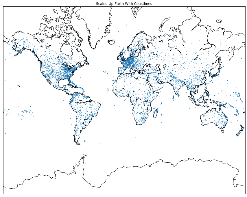
We create a visualization on world airports.
from mpl_toolkits.basemap import Basemap
m = Basemap(projection='merc',llcrnrlat=-80,urcrnrlat=80,llcrnrlon=-180,urcrnrlon=180)
longitudes = airports["longitude"].tolist()
latitudes = airports["latitude"].tolist()
x, y = m(longitudes, latitudes)
fig, ax = plt.subplots(figsize=(10,15))
plt.title("Scaled Up Earth With Coastlines")
m.scatter(x,y,s=1)
m.drawcoastlines()
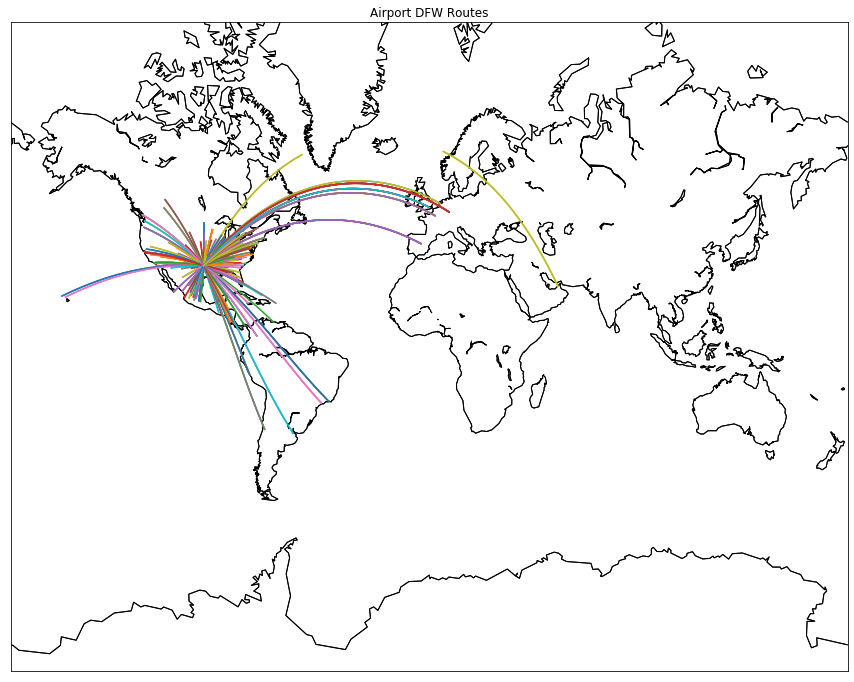
We also created a visualization of one sample airport which includes its flight routes.
geo_routes = pd.read_csv('geo_routes.csv')
geo_routes
| airline | source | dest | equipment | start_lon | end_lon | start_lat | end_lat | |
|---|---|---|---|---|---|---|---|---|
| 0 | 2B | AER | KZN | CR2 | 39.956589 | 49.278728 | 43.449928 | 55.606186 |
| 1 | 2B | ASF | KZN | CR2 | 48.006278 | 49.278728 | 46.283333 | 55.606186 |
| 2 | 2B | ASF | MRV | CR2 | 48.006278 | 43.081889 | 46.283333 | 44.225072 |
| 3 | 2B | CEK | KZN | CR2 | 61.503333 | 49.278728 | 55.305836 | 55.606186 |
| 4 | 2B | CEK | OVB | CR2 | 61.503333 | 82.650656 | 55.305836 | 55.012622 |
| ... | ... | ... | ... | ... | ... | ... | ... | ... |
| 67423 | ZL | WYA | ADL | SF3 | 137.514000 | 138.530556 | -33.058900 | -34.945000 |
| 67424 | ZM | DME | FRU | 734 | 37.906111 | 74.477556 | 55.408611 | 43.061306 |
| 67425 | ZM | FRU | DME | 734 | 74.477556 | 37.906111 | 43.061306 | 55.408611 |
| 67426 | ZM | FRU | OSS | 734 | 74.477556 | 72.793269 | 43.061306 | 40.608989 |
| 67427 | ZM | OSS | FRU | 734 | 72.793269 | 74.477556 | 40.608989 | 43.061306 |
67428 rows × 8 columns
# a helper function that that draws a great circle for each route that has an absolute difference in the latitude and longitude values less than 180.
def create_great_circles(df):
    for index, row in df.iterrows():
        end_lat, start_lat = row['end_lat'], row['start_lat']
        end_lon, start_lon = row['end_lon'], row['start_lon']

        if abs(end_lat - start_lat) < 180:
            if abs(end_lon - start_lon) < 180:
                m.drawgreatcircle(start_lon, start_lat, end_lon, end_lat)
fig, ax = plt.subplots(figsize=(10,15))
m = Basemap(projection='merc', llcrnrlat=-80, urcrnrlat=80, llcrnrlon=-180, urcrnrlon=180)
m.drawcoastlines()
plt.title("Airport DFW Routes")
dfw = geo_routes[geo_routes['source'] == "DFW"]
create_great_circles(dfw)
m.drawcoastlines()
plt.show()