Dimensionality Reduction: 1000 fashion MNIST

Goals

1. Try out different Dimensionality Reduction (DR) techniques, and choose the best: TNSE

2. DR for Pre-processing: not very favourable

Data set description

Source: https://github.com/zalandoresearch/fashion-mnist

Fashion-MNIST is a dataset of Zalando’s article images—consisting of a training set of 60,000 examples and a test set of 10,000 examples. Each example is a 28x28 grayscale image, associated with a label from 10 classes. Zalando intends Fashion-MNIST to serve as a direct drop-in replacement for the original MNIST dataset for benchmarking machine learning algorithms. It shares the same image size and structure of training and testing splits.

Each image is 28 pixels in height and 28 pixels in width, for a total of 784 pixels in total. Each pixel has a single pixel-value associated with it, indicating the lightness or darkness of that pixel, with higher numbers meaning darker. This pixel-value is an integer between 0 and 255. The training and test data sets have 785 columns. The first column consists of the class labels (see above), and represents the article of clothing. The rest of the columns contain the pixel-values of the associated image.

Attributes

• 0: T-shirt/top
• 1: Trouser
• 2: Pullover
• 3: Dress
• 4: Coat
• 5: Sandal
• 6: Shirt
• 7: Sneaker
• 8: Bag
• 9: Ankle boot

ML tasks

1. Perform Dimentionality Reduction (DR) techniques
2. Classification with DR as Pre-processing

We’ll use 1000 rows from the original dataset only.

import pandas as pd

data = pd.read_csv('fashion-mnist.csv')
data

	label	pixel1	pixel2	pixel3	pixel4	pixel5	pixel6	pixel7	pixel8	pixel9	...	pixel775	pixel776	pixel777	pixel778	pixel779	pixel780	pixel781	pixel782	pixel783	pixel784
0	0	0	0	0	0	0	0	0	9	8	...	103	87	56	0	0	0	0	0	0	0
1	1	0	0	0	0	0	0	0	0	0	...	34	0	0	0	0	0	0	0	0	0
2	2	0	0	0	0	0	0	14	53	99	...	0	0	0	0	63	53	31	0	0	0
3	2	0	0	0	0	0	0	0	0	0	...	137	126	140	0	133	224	222	56	0	0
4	3	0	0	0	0	0	0	0	0	0	...	0	0	0	0	0	0	0	0	0	0
...	...	...	...	...	...	...	...	...	...	...	...	...	...	...	...	...	...	...	...	...	...
9995	0	0	0	0	0	0	0	0	0	0	...	32	23	14	20	0	0	1	0	0	0
9996	6	0	0	0	0	0	0	0	0	0	...	0	0	0	2	52	23	28	0	0	0
9997	8	0	0	0	0	0	0	0	0	0	...	175	172	172	182	199	222	42	0	1	0
9998	8	0	1	3	0	0	0	0	0	0	...	0	0	0	0	0	1	0	0	0	0
9999	1	0	0	0	0	0	0	0	140	119	...	111	95	75	44	1	0	0	0	0	0

10000 rows × 785 columns

from sklearn.model_selection import train_test_split

X, y = data.iloc[:, 1:].to_numpy(), data.iloc[:, 0].to_numpy()
X_train, X_test, y_train, y_test = train_test_split(X, y, test_size=0.33, random_state=42)

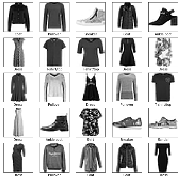
class_names = ['T-shirt/top', 'Trouser', 'Pullover', 'Dress', 'Coat',
               'Sandal', 'Shirt', 'Sneaker', 'Bag', 'Ankle boot']

import matplotlib.pyplot as plt

plt.figure(figsize=(10,10))
for i in range(25):
    plt.subplot(5,5,i+1)
    plt.xticks([])
    plt.yticks([])
    plt.grid(False)
    plt.imshow(X_train[i].reshape(28, 28), cmap="binary")
    plt.xlabel(class_names[y_train[i]])
plt.show()

1.1. PCA

# perform PCA and keep 95% of variance

from sklearn.decomposition import PCA

pca = PCA(n_components = 0.95)
X_reduced = pca.fit_transform(X_train)

Most variance lies along the first two principal components

pca.explained_variance_ratio_[:10]

array([0.28701888, 0.18049693, 0.05945456, 0.04980945, 0.03838398,
       0.03475959, 0.02353651, 0.01864746, 0.0139102 , 0.01324683])

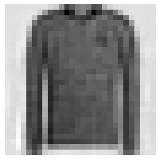
# reconstruct data from compressed data

pca = PCA(n_components = 179)
X_reduced = pca.fit_transform(X_train)
X_recovered = pca.inverse_transform(X_reduced)

import matplotlib as mpl
import matplotlib.pyplot as plt

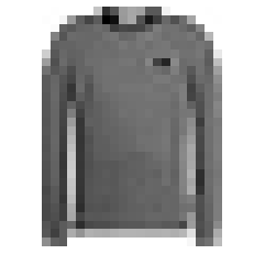
print('non-compressed image')
plt.imshow(X_train[100].reshape(28, 28), cmap="binary")
plt.axis("off")
plt.show()

non-compressed image

print('95% variance compressed image')
plt.imshow(X_recovered[100].reshape(28, 28), cmap="binary")
plt.axis("off")
plt.show()

95% variance compressed image

# helper function for plotting

from sklearn.preprocessing import MinMaxScaler
from matplotlib.offsetbox import AnnotationBbox, OffsetImage
import numpy as np

def plot_digits(X, y, min_distance=0.05, images=None, figsize=(13, 10)):
    # Let's scale the input features so that they range from 0 to 1
    X_normalized = MinMaxScaler().fit_transform(X)
    # Now we create the list of coordinates of the digits plotted so far.
    # We pretend that one is already plotted far away at the start, to
    # avoid `if` statements in the loop below
    neighbors = np.array([[10., 10.]])
    # The rest should be self-explanatory
    plt.figure(figsize=figsize)
    cmap = mpl.cm.get_cmap("prism")
    digits = np.unique(y)
    for digit in digits:
        plt.scatter(X_normalized[y == digit, 0], X_normalized[y == digit, 1], c=[cmap(digit / 9)])
    plt.axis("off")
    ax = plt.gcf().gca()  # get current axes in current figure
    for index, image_coord in enumerate(X_normalized):
        closest_distance = np.linalg.norm(np.array(neighbors) - image_coord, axis=1).min()
        if closest_distance > min_distance:
            neighbors = np.r_[neighbors, [image_coord]]
            if images is None:
                plt.text(image_coord[0], image_coord[1], str(int(y[index])),
                         color=cmap(y[index] / 9), fontdict={"weight": "bold", "size": 16})
            else:
                image = images[index].reshape(28, 28)
                imagebox = AnnotationBbox(OffsetImage(image, cmap="binary"), image_coord)
                ax.add_artist(imagebox)

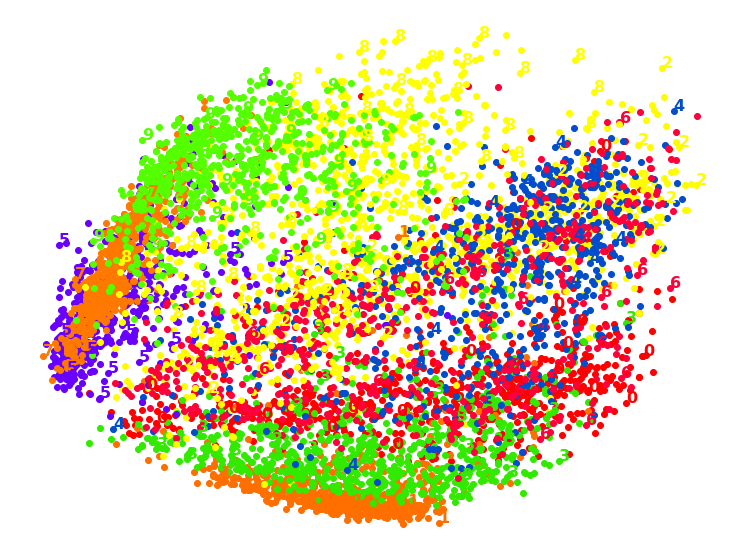
X_pca_reduced = PCA(n_components=2, random_state=42).fit_transform(X_train)
plot_digits(X_pca_reduced, y_train)
plt.show()

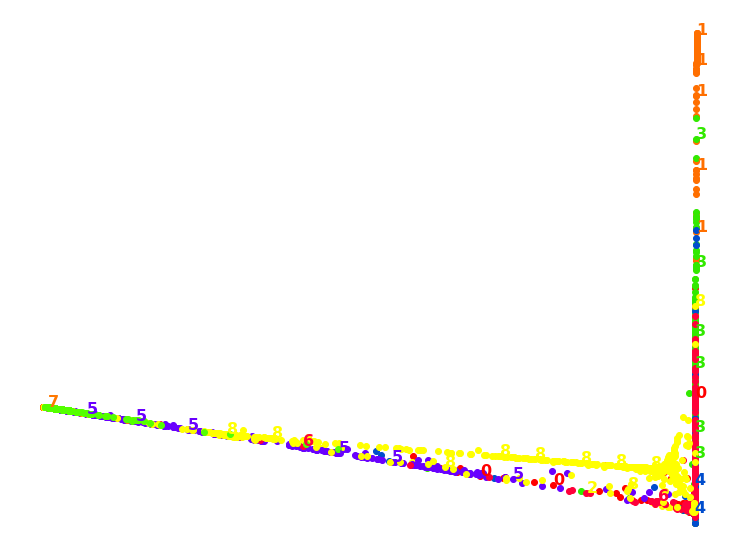
1.2. LDA

from sklearn.discriminant_analysis import LinearDiscriminantAnalysis

X_lda_reduced = LinearDiscriminantAnalysis(n_components=2).fit_transform(X_train, y_train)
plot_digits(X_lda_reduced, y_train, figsize=(12,12))
plt.show()

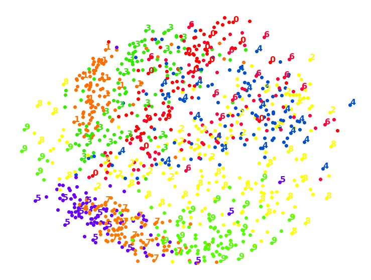
1.3. LLE

from sklearn.pipeline import Pipeline
from sklearn.manifold import LocallyLinearEmbedding

pca_lle = Pipeline([
    ("pca", PCA(n_components=0.95, random_state=42)),
    ("lle", LocallyLinearEmbedding(n_components=2, random_state=42)),
])
X_pca_lle_reduced = pca_lle.fit_transform(X_train)
plot_digits(X_pca_lle_reduced, y_train)
plt.show()

1.4. MDS

from sklearn.manifold import MDS

pca_mds = Pipeline([
    ("pca", PCA(n_components=0.95, random_state=42)),
    ("mds", MDS(n_components=2, random_state=42)),
])
X_pca_mds_reduced = pca_mds.fit_transform(X_train[:1000])
plot_digits(X_pca_mds_reduced, y_train[:1000])
plt.show()

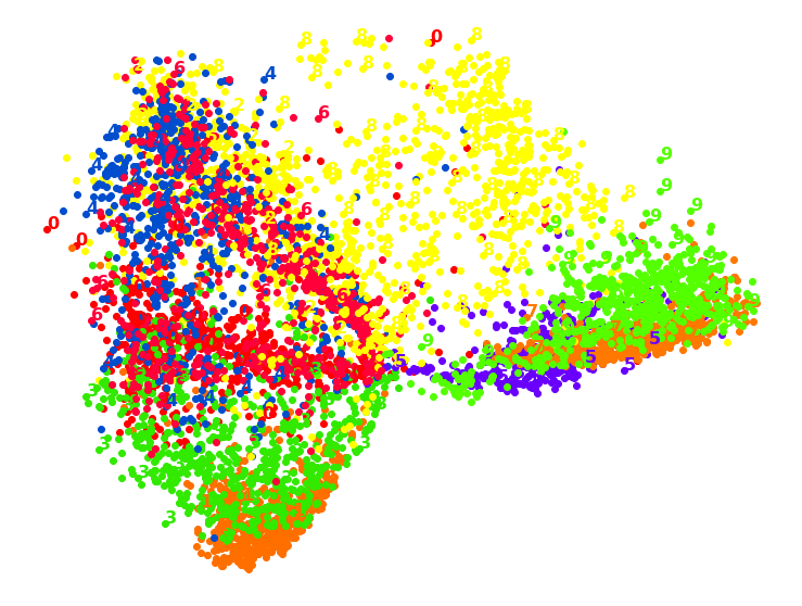
1.5. Isomap

from sklearn.manifold import Isomap

pca_isomap = Pipeline([
    ("pca", PCA(n_components=0.95, random_state=42)),
    ("isomap", Isomap(n_components=2)),
])
X_pca_isomap_reduced = pca_isomap.fit_transform(X_train)
plot_digits(X_pca_isomap_reduced, y_train)
plt.show()

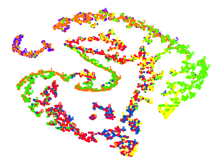
1.6. TSNE

from sklearn.manifold import TSNE

pca_tsne = Pipeline([
    ("pca", PCA(n_components=0.95, random_state=42)),
    ("tsne", TSNE(n_components=2, random_state=42)),
])
X_pca_tsne_reduced = pca_tsne.fit_transform(X_train)
plot_digits(X_pca_tsne_reduced, y_train)
plt.show()

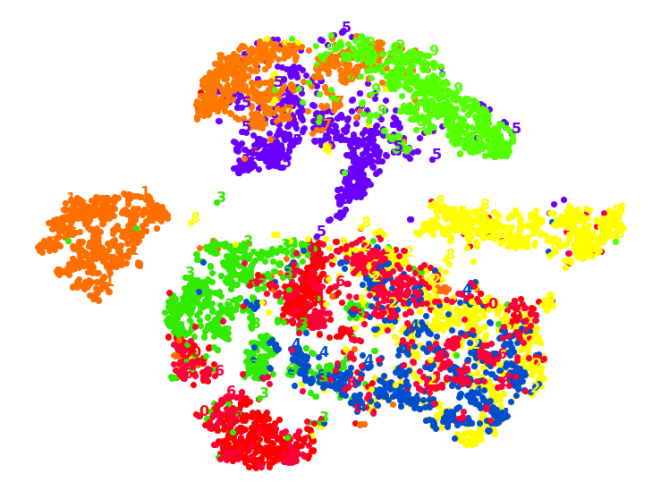
TSNS gives the clearest distinction between classes.

1.7. TSNE with ‘rbf’ KPCA

from sklearn.decomposition import KernelPCA
from sklearn.manifold import TSNE

k_pca_tsne = Pipeline([
    ("kpca", KernelPCA(n_components=2, kernel='rbf', random_state=42)),
    ("tsne", TSNE(n_components=2, random_state=42)),
])
X_pca_tsne_reduced = k_pca_tsne.fit_transform(X_train)
plot_digits(X_pca_tsne_reduced, y_train)
plt.show()

1.8. TSNE with ‘poly’ KPCA

k_pca_tsne = Pipeline([
    ("kpca", KernelPCA(n_components=2, kernel='poly', random_state=42)),
    ("tsne", TSNE(n_components=2, random_state=42)),
])
X_pca_tsne_reduced = k_pca_tsne.fit_transform(X_train)
plot_digits(X_pca_tsne_reduced, y_train)
plt.show()

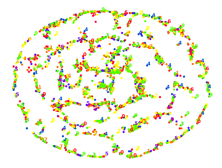
1.9. TSNE with ‘sigmoid’ PCA

k_pca_tsne = Pipeline([
    ("kpca", KernelPCA(n_components=2, kernel='sigmoid', random_state=42)),
    ("tsne", TSNE(n_components=2, random_state=42)),
])
X_pca_tsne_reduced = k_pca_tsne.fit_transform(X_train)
plot_digits(X_pca_tsne_reduced, y_train)
plt.show()

2.1. Classification with PCA and TNSE

from sklearn.linear_model import LogisticRegression

lr = LogisticRegression()
lr.fit(X_pca_tsne_reduced, y_train)

LogisticRegression(C=1.0, class_weight=None, dual=False, fit_intercept=True,
                   intercept_scaling=1, l1_ratio=None, max_iter=100,
                   multi_class='auto', n_jobs=None, penalty='l2',
                   random_state=None, solver='lbfgs', tol=0.0001, verbose=0,
                   warm_start=False)

pca_tsne = Pipeline([
    ("pca", PCA(n_components=0.95, random_state=42)),
    ("tsne", TSNE(n_components=2, random_state=42)),
])
X_pca_tsne_reduced_test = pca_tsne.fit_transform(X_test)

from sklearn.metrics import accuracy_score

accuracy_score(y_test, lr.predict(X_pca_tsne_reduced_test))

0.0048484848484848485

The result is very bad. So we can try simple PCA with 2 components.

lr = LogisticRegression(max_iter=100000)
lr.fit(X_pca_reduced, y_train)

LogisticRegression(C=1.0, class_weight=None, dual=False, fit_intercept=True,
                   intercept_scaling=1, l1_ratio=None, max_iter=100000,
                   multi_class='auto', n_jobs=None, penalty='l2',
                   random_state=None, solver='lbfgs', tol=0.0001, verbose=0,
                   warm_start=False)

X_pca_reduced_test = PCA(n_components=2, random_state=42).fit_transform(X_test)

accuracy_score(y_test, lr.predict(X_pca_reduced_test))

0.5130303030303031

This is still not the accuracy we expect, so it is not a good idea to try PCA with 2 components.