My Bui (Mimi)
Data Engineer & DataOps
My LinkedIn
My GitHub
QWERTY keyboard typing with 1 finger: modeling and analysis using Fiit’s law and Zipf’s law
Goals
1. Modeling the keyboard
2. Fiit’s law parameter estimation: r-squared = 0.709
3. Average typing time of 1000 most frequent words: 0.99
4. Zipf’s law parameter estimation & average typing time of 1000 most frequent words: 0.71
import matplotlib.pyplot as plt
import math
import numpy
numpy.set_printoptions(precision=2)
import scipy.stats as stats
import statsmodels.api as sm
from statsmodels.graphics.regressionplots import abline_plot
import seaborn as sns
1. Keyboard modeling
# Define keyboard
line1 = 'qwertyuiop'
line2 = 'asdfghjkl'
line3 = 'zxcvbnm'

# Define a keyboard as a list of keys.
# Each key also mentions its position in the keyboard (line number, column number)
keyboard  = [(i, (0, ni)) for ni, i in enumerate(line1)] + [(i, (1, ni)) for ni, i in enumerate(line2)] + [(i, (2, ni)) for ni, i in enumerate(line3)]

# Define empty matrices to hold the results
ids = numpy.zeros((26, 26))
Ds = numpy.zeros((26, 26))
W = 1

alphabet = line1 + line2 + line3
Fitts’ law predicts the time MT required to select a target of size W that is located D away: $MT = a + b\cdot\log_{2}\left ( 1+\frac{D}{W} \right )$, where ID = $\log_{2}\left ( 1+\frac{D}{W} \right )$ is the index of difficulty
# Get the index of difficulty (ID) for each key combination
for ns, keystart in enumerate(alphabet):
    for ne, keyend in enumerate(alphabet):
        xs, ys, xe, ye = keyboard[ns][1][1] + 2/5*keyboard[ns][1][0], keyboard[ns][1][0], keyboard[ne][1][1] + 2/5*keyboard[ne][1][0], keyboard[ne][1][0]
        # Compute euclidian distance between the startkey and endkey
        D = math.sqrt((xe - xs)**2 + (ye - ys)**2)
        Ds[ns, ne] = D
        # Use Fitts' law formula
        ids[ns, ne] = math.log2(1 + D/W)
ids
array([[0.  , 1.  , 1.58, 2.  , 2.32, 2.58, 2.81, 3.  , 3.17, 3.32, 1.05,
        1.44, 1.85, 2.18, 2.46, 2.7 , 2.9 , 3.08, 3.24, 1.66, 1.88, 2.15,
        2.4 , 2.63, 2.83, 3.02],
       [1.  , 0.  , 1.  , 1.58, 2.  , 2.32, 2.58, 2.81, 3.  , 3.17, 1.12,
        1.05, 1.44, 1.85, 2.18, 2.46, 2.7 , 2.9 , 3.08, 1.59, 1.66, 1.88,
        2.15, 2.4 , 2.63, 2.83],
       [1.58, 1.  , 0.  , 1.  , 1.58, 2.  , 2.32, 2.58, 2.81, 3.  , 1.53,
        1.12, 1.05, 1.44, 1.85, 2.18, 2.46, 2.7 , 2.9 , 1.74, 1.59, 1.66,
        1.88, 2.15, 2.4 , 2.63],
       [2.  , 1.58, 1.  , 0.  , 1.  , 1.58, 2.  , 2.32, 2.58, 2.81, 1.92,
        1.53, 1.12, 1.05, 1.44, 1.85, 2.18, 2.46, 2.7 , 1.99, 1.74, 1.59,
        1.66, 1.88, 2.15, 2.4 ],
       [2.32, 2.  , 1.58, 1.  , 0.  , 1.  , 1.58, 2.  , 2.32, 2.58, 2.24,
        1.92, 1.53, 1.12, 1.05, 1.44, 1.85, 2.18, 2.46, 2.26, 1.99, 1.74,
        1.59, 1.66, 1.88, 2.15],
       [2.58, 2.32, 2.  , 1.58, 1.  , 0.  , 1.  , 1.58, 2.  , 2.32, 2.51,
        2.24, 1.92, 1.53, 1.12, 1.05, 1.44, 1.85, 2.18, 2.5 , 2.26, 1.99,
        1.74, 1.59, 1.66, 1.88],
       [2.81, 2.58, 2.32, 2.  , 1.58, 1.  , 0.  , 1.  , 1.58, 2.  , 2.74,
        2.51, 2.24, 1.92, 1.53, 1.12, 1.05, 1.44, 1.85, 2.72, 2.5 , 2.26,
        1.99, 1.74, 1.59, 1.66],
       [3.  , 2.81, 2.58, 2.32, 2.  , 1.58, 1.  , 0.  , 1.  , 1.58, 2.94,
        2.74, 2.51, 2.24, 1.92, 1.53, 1.12, 1.05, 1.44, 2.91, 2.72, 2.5 ,
        2.26, 1.99, 1.74, 1.59],
       [3.17, 3.  , 2.81, 2.58, 2.32, 2.  , 1.58, 1.  , 0.  , 1.  , 3.12,
        2.94, 2.74, 2.51, 2.24, 1.92, 1.53, 1.12, 1.05, 3.08, 2.91, 2.72,
        2.5 , 2.26, 1.99, 1.74],
       [3.32, 3.17, 3.  , 2.81, 2.58, 2.32, 2.  , 1.58, 1.  , 0.  , 3.27,
        3.12, 2.94, 2.74, 2.51, 2.24, 1.92, 1.53, 1.12, 3.24, 3.08, 2.91,
        2.72, 2.5 , 2.26, 1.99],
       [1.05, 1.12, 1.53, 1.92, 2.24, 2.51, 2.74, 2.94, 3.12, 3.27, 0.  ,
        1.  , 1.58, 2.  , 2.32, 2.58, 2.81, 3.  , 3.17, 1.05, 1.44, 1.85,
        2.18, 2.46, 2.7 , 2.9 ],
       [1.44, 1.05, 1.12, 1.53, 1.92, 2.24, 2.51, 2.74, 2.94, 3.12, 1.  ,
        0.  , 1.  , 1.58, 2.  , 2.32, 2.58, 2.81, 3.  , 1.12, 1.05, 1.44,
        1.85, 2.18, 2.46, 2.7 ],
       [1.85, 1.44, 1.05, 1.12, 1.53, 1.92, 2.24, 2.51, 2.74, 2.94, 1.58,
        1.  , 0.  , 1.  , 1.58, 2.  , 2.32, 2.58, 2.81, 1.53, 1.12, 1.05,
        1.44, 1.85, 2.18, 2.46],
       [2.18, 1.85, 1.44, 1.05, 1.12, 1.53, 1.92, 2.24, 2.51, 2.74, 2.  ,
        1.58, 1.  , 0.  , 1.  , 1.58, 2.  , 2.32, 2.58, 1.92, 1.53, 1.12,
        1.05, 1.44, 1.85, 2.18],
       [2.46, 2.18, 1.85, 1.44, 1.05, 1.12, 1.53, 1.92, 2.24, 2.51, 2.32,
        2.  , 1.58, 1.  , 0.  , 1.  , 1.58, 2.  , 2.32, 2.24, 1.92, 1.53,
        1.12, 1.05, 1.44, 1.85],
       [2.7 , 2.46, 2.18, 1.85, 1.44, 1.05, 1.12, 1.53, 1.92, 2.24, 2.58,
        2.32, 2.  , 1.58, 1.  , 0.  , 1.  , 1.58, 2.  , 2.51, 2.24, 1.92,
        1.53, 1.12, 1.05, 1.44],
       [2.9 , 2.7 , 2.46, 2.18, 1.85, 1.44, 1.05, 1.12, 1.53, 1.92, 2.81,
        2.58, 2.32, 2.  , 1.58, 1.  , 0.  , 1.  , 1.58, 2.74, 2.51, 2.24,
        1.92, 1.53, 1.12, 1.05],
       [3.08, 2.9 , 2.7 , 2.46, 2.18, 1.85, 1.44, 1.05, 1.12, 1.53, 3.  ,
        2.81, 2.58, 2.32, 2.  , 1.58, 1.  , 0.  , 1.  , 2.94, 2.74, 2.51,
        2.24, 1.92, 1.53, 1.12],
       [3.24, 3.08, 2.9 , 2.7 , 2.46, 2.18, 1.85, 1.44, 1.05, 1.12, 3.17,
        3.  , 2.81, 2.58, 2.32, 2.  , 1.58, 1.  , 0.  , 3.12, 2.94, 2.74,
        2.51, 2.24, 1.92, 1.53],
       [1.66, 1.59, 1.74, 1.99, 2.26, 2.5 , 2.72, 2.91, 3.08, 3.24, 1.05,
        1.12, 1.53, 1.92, 2.24, 2.51, 2.74, 2.94, 3.12, 0.  , 1.  , 1.58,
        2.  , 2.32, 2.58, 2.81],
       [1.88, 1.66, 1.59, 1.74, 1.99, 2.26, 2.5 , 2.72, 2.91, 3.08, 1.44,
        1.05, 1.12, 1.53, 1.92, 2.24, 2.51, 2.74, 2.94, 1.  , 0.  , 1.  ,
        1.58, 2.  , 2.32, 2.58],
       [2.15, 1.88, 1.66, 1.59, 1.74, 1.99, 2.26, 2.5 , 2.72, 2.91, 1.85,
        1.44, 1.05, 1.12, 1.53, 1.92, 2.24, 2.51, 2.74, 1.58, 1.  , 0.  ,
        1.  , 1.58, 2.  , 2.32],
       [2.4 , 2.15, 1.88, 1.66, 1.59, 1.74, 1.99, 2.26, 2.5 , 2.72, 2.18,
        1.85, 1.44, 1.05, 1.12, 1.53, 1.92, 2.24, 2.51, 2.  , 1.58, 1.  ,
        0.  , 1.  , 1.58, 2.  ],
       [2.63, 2.4 , 2.15, 1.88, 1.66, 1.59, 1.74, 1.99, 2.26, 2.5 , 2.46,
        2.18, 1.85, 1.44, 1.05, 1.12, 1.53, 1.92, 2.24, 2.32, 2.  , 1.58,
        1.  , 0.  , 1.  , 1.58],
       [2.83, 2.63, 2.4 , 2.15, 1.88, 1.66, 1.59, 1.74, 1.99, 2.26, 2.7 ,
        2.46, 2.18, 1.85, 1.44, 1.05, 1.12, 1.53, 1.92, 2.58, 2.32, 2.  ,
        1.58, 1.  , 0.  , 1.  ],
       [3.02, 2.83, 2.63, 2.4 , 2.15, 1.88, 1.66, 1.59, 1.74, 1.99, 2.9 ,
        2.7 , 2.46, 2.18, 1.85, 1.44, 1.05, 1.12, 1.53, 2.81, 2.58, 2.32,
        2.  , 1.58, 1.  , 0.  ]])
2. Fiit’s law parameter estimation
# This function opens the file, and reads the startkey, endkey, and duration of each typing stroke
# and returns the index of difficulty ID, and time required
def get_keystrokes(filename, ids):
    ID, MT = [], []
    with open(filename, 'r') as _file:
        startime = 0
        for n, line in enumerate(_file):
            #print(n, line)
            try:
                startkey, stopkey, time = line.split(",")
                #print(startkey, stopkey, time)
                time = float(time.rsplit('\n')[0])
                # if startkey == 'None':
                if n == 0:
                    startime = time
                    continue
                startkey = startkey.split("'")[1]
                stopkey = stopkey.split("'")[1]
                if startkey not in alphabet or stopkey not in alphabet:
                    continue
                ns = alphabet.index(startkey)
                ne = alphabet.index(stopkey)
                mt = time - startime
                MT.append(mt)
                ID.append(ids[ns, ne])
                startime = time
            except IndexError:
                pass

    return ID, MT
# Estimate the parameters of Fitts' law
def analyse_keystrokes(ID, MT, ax):
    ax.plot(ID, MT, 'o')
    X = ID
    y = MT
    X = sm.add_constant(X)
    model = sm.OLS(y, X).fit()
    predictions = model.predict(X)

    print(model.summary())
    abline_plot(model_results=model, ax=ax)

    return (model.rsquared, model.conf_int())
View of the file
import pandas as pd

pd.read_csv('keystrokes.csv')
| None | 't' | 1603459783.882251 | |
|---|---|---|---|
| 0 | 't' | 'h' | 1.603460e+09 |
| 1 | 'h' | 'e' | 1.603460e+09 |
| 2 | 'e' | 'b' | 1.603460e+09 |
| 3 | 'b' | 'r' | 1.603460e+09 |
| 4 | 'r' | 'o' | 1.603460e+09 |
| 5 | 'o' | 'w' | 1.603460e+09 |
| 6 | 'w' | 'n' | 1.603460e+09 |
| 7 | 'n' | 'f' | 1.603460e+09 |
| 8 | 'f' | 'o' | 1.603460e+09 |
| 9 | 'o' | 'x' | 1.603460e+09 |
| 10 | 'x' | 'j' | 1.603460e+09 |
| 11 | 'j' | 'u' | 1.603460e+09 |
| 12 | 'u' | 'm' | 1.603460e+09 |
| 13 | 'm' | 'p' | 1.603460e+09 |
| 14 | 'p' | 's' | 1.603460e+09 |
| 15 | 's' | 'o' | 1.603460e+09 |
| 16 | 'o' | 'v' | 1.603460e+09 |
| 17 | 'v' | 'e' | 1.603460e+09 |
| 18 | 'e' | 'r' | 1.603460e+09 |
| 19 | 'r' | 't' | 1.603460e+09 |
| 20 | 't' | 'h' | 1.603460e+09 |
| 21 | 'h' | 'e' | 1.603460e+09 |
| 22 | 'e' | 'g' | 1.603460e+09 |
| 23 | 'g' | 'r' | 1.603460e+09 |
| 24 | 'r' | 'a' | 1.603460e+09 |
| 25 | 'a' | 'y' | 1.603460e+09 |
| 26 | 'y' | 'd' | 1.603460e+09 |
| 27 | 'd' | 'o' | 1.603460e+09 |
| 28 | 'o' | 'g' | 1.603460e+09 |
| 29 | 'g' | Key.esc | 1.603460e+09 |
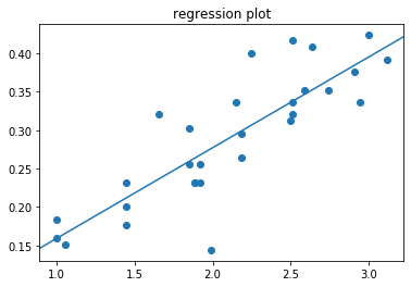
# How well Fitts' model fits: graphical representation, a goodness of fit of choice, and the uncertainty with regards to estimated parameters
fig = plt.figure()
ax = fig.add_subplot(111)
ID, MT = get_keystrokes('keystrokes.csv', ids)
analyse_keystrokes(ID, MT, ax)
ax.set_title('regression plot')
plt.show()
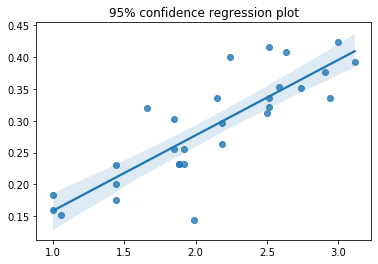
fig = plt.figure()
ax = fig.add_subplot(111)
sns.regplot(x=ID, y=MT, x_ci='ci', ci=95)
ax.set_title('95% confidence regression plot')
plt.show()
                            OLS Regression Results
==============================================================================
Dep. Variable:                      y   R-squared:                       0.709
Model:                            OLS   Adj. R-squared:                  0.698
Method:                 Least Squares   F-statistic:                     65.63
Date:                Mon, 02 Nov 2020   Prob (F-statistic):           1.05e-08
Time:                        12:52:49   Log-Likelihood:                 48.860
No. Observations:                  29   AIC:                            -93.72
Df Residuals:                      27   BIC:                            -90.99
Df Model:                           1
Covariance Type:            nonrobust
==============================================================================
                 coef    std err          t      P>|t|      [0.025      0.975]
------------------------------------------------------------------------------
const          0.0404      0.032      1.265      0.217      -0.025       0.106
x1             0.1184      0.015      8.101      0.000       0.088       0.148
==============================================================================
Omnibus:                        3.192   Durbin-Watson:                   2.125
Prob(Omnibus):                  0.203   Jarque-Bera (JB):                2.001
Skew:                          -0.150   Prob(JB):                        0.368
Kurtosis:                       4.251   Cond. No.                         9.68
==============================================================================

Warnings:
[1] Standard Errors assume that the covariance matrix of the errors is correctly specified.
3. Average typing time of 1000 most frequent words
View of the file
pd.read_csv('mostcommonwords.txt')
| the | |
|---|---|
| 0 | of |
| 1 | to |
| 2 | and |
| 3 | a |
| 4 | in |
| ... | ... |
| 994 | meant |
| 995 | quotient |
| 996 | teeth |
| 997 | shell |
| 998 | neck |
999 rows × 1 columns
# Most Common words
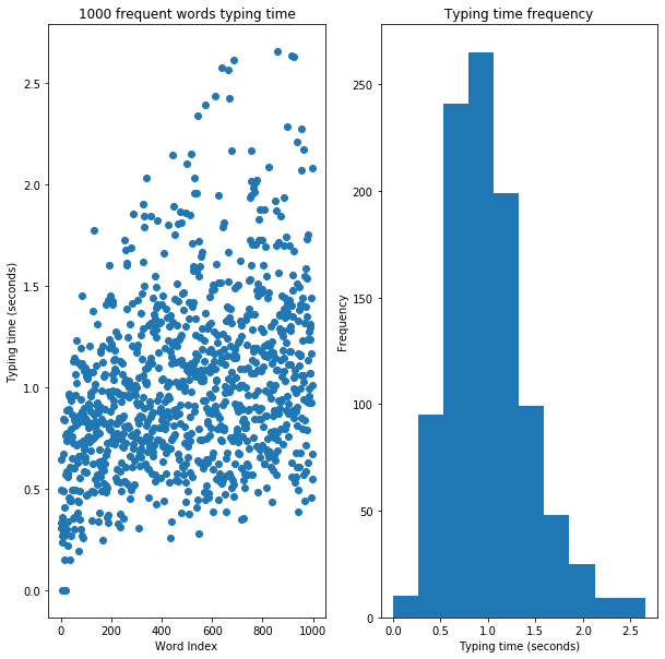
# Estimate the average time needed to type the 1000 most common english words
# These words are given in the accompanying mostcommonwords.txt file.
# No information of frequency is given, so assume that each word is equally probable
# Consider that the first key is "free", i.e. time starts only after the first key of the word is pressed
slope = 0.12
intercept = 0.03
with open("mostcommonwords.txt", 'r') as _file:
T = []
for nline, line in enumerate(_file):
t = 0
line = line[:-1]
#print(line, len(line))
for i in range(0, len(line)-1):
try:
ns = alphabet.index(line[i])
ne = alphabet.index(line[i+1])
id = ids[ns, ne]
t += intercept + (slope*id)
except ValueError:
pass
T.append(t)
print("Average time needed")
print(numpy.mean(T))
Average time needed
0.9999165686462256
fig = plt.figure(figsize=(10, 10))
ax = fig.add_subplot(121)
axhist = fig.add_subplot(122)

ax.plot(range(0,len(T)), T, 'o')
ax.set_ylabel("Typing time (seconds)")
ax.set_xlabel("Word Index")
ax.set_title('1000 frequent words typing time')
axhist.hist(T)
axhist.set_xlabel("Typing time (seconds)")
axhist.set_ylabel("Frequency")
axhist.set_title('Typing time frequency')
plt.show()
plt.close()
4. Zipf’s law parameter estimation & average typing time of 1000 most frequent words
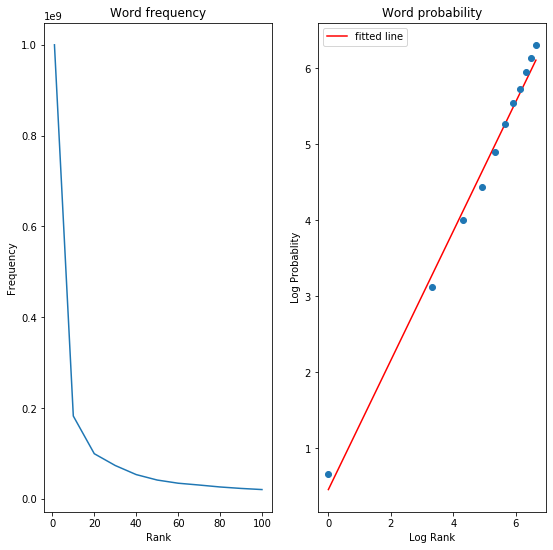
Zipf’s law states that the frequency of a word is inversely proportional to its rank in the frequency table: $p(k) = \frac{\frac{1}{k^{s}}}{\sum 1/i^{s}}$
# Modeling word frequency
# Frenquency/occurence pairs for the 100 most frequent english words to estimate s of Zipf's model
frequency = [1e9, 182e6, 99e6, 73e6, 53e6, 41e6, 34e6, 30e6, 25.7e6, 22.5e6, 20e6]
rank  = [1, 10, 20, 30, 40, 50, 60, 70, 80, 90, 100]

logfreq = [math.log(f, 2) for f in frequency]
logoc = [math.log(o, 2) for o in rank]

# Fit Zipf's model to the frequencey-rank relationship
prob = numpy.array(frequency)/sum(frequency)
logprob = numpy.array([math.log(f, 2) for f in prob]) * (-1)

slope, intercept, r_value, p_value, std_err = stats.linregress(logoc, logprob)
s = round(slope, 2)
## Plot the data + fitted model
fig = plt.figure(figsize=(9, 9))
ax = fig.add_subplot(121)
axlog = fig.add_subplot(122)
ax.plot(rank, frequency, '-')
ax.set_title('Word frequency')
ax.set_xlabel("Rank")
ax.set_ylabel("Frequency")

axlog.plot(logoc, intercept + s*(numpy.array(logoc)), 'r', label='fitted line')
axlog.plot(logoc, logprob, 'o')
axlog.set_title('Word probability')
axlog.set_xlabel("Log Rank")
axlog.set_ylabel("Log Probablity")
plt.legend()
plt.show()
## Use this new information to evaluate the average time it takes to type the 1000 most common words
_sum = sum([1/(i**s) for i in list(range(1, 1001))])

# Compute the p(k)'s for each k
weights = []
for nt in range(1, 1001):
    weight = (1/(nt**s))/_sum
    weights.append(weight)

weighted_sum = 0
for w,t in zip(weights, T):
    weighted_sum += w*t

print(weighted_sum)
0.7124495668649804