This data set explores the relationship between income and religion in the US. It comes from a report produced by the Pew Research Center, an American think-tank that collects data on attitudes to topics ranging from religion to the internet.

import pandas as pd
import numpy as np
import seaborn as sns
import matplotlib.pyplot as plt

%matplotlib inline

pew_data = pd.read_csv('Data/pew.csv')
pew_data

	religion	<$10k	$10-20k	$20-30k	$30-40k	$40-50k	$50-75k	$75-100k	$100-150k	>150k	Don't know/refused
0	Agnostic	27	34	60	81	76	137	122	109	84	96
1	Atheist	12	27	37	52	35	70	73	59	74	76
2	Buddhist	27	21	30	34	33	58	62	39	53	54
3	Catholic	418	617	732	670	638	1116	949	792	633	1489
4	Don’t know/refused	15	14	15	11	10	35	21	17	18	116
5	Evangelical Prot	575	869	1064	982	881	1486	949	723	414	1529
6	Hindu	1	9	7	9	11	34	47	48	54	37
7	Historically Black Prot	228	244	236	238	197	223	131	81	78	339
8	Jehovah's Witness	20	27	24	24	21	30	15	11	6	37
9	Jewish	19	19	25	25	30	95	69	87	151	162
10	Mainline Prot	289	495	619	655	651	1107	939	753	634	1328
11	Mormon	29	40	48	51	56	112	85	49	42	69
12	Muslim	6	7	9	10	9	23	16	8	6	22
13	Orthodox	13	17	23	32	32	47	38	42	46	73
14	Other Christian	9	7	11	13	13	14	18	14	12	18
15	Other Faiths	20	33	40	46	49	63	46	40	41	71
16	Other World Religions	5	2	3	4	2	7	3	4	4	8
17	Unaffiliated	217	299	374	365	341	528	407	321	258	597

pew_data['Total'] = pew_data.sum(axis=1)
pew_data.set_index('religion', inplace=True)
pew_data

	<$10k	$10-20k	$20-30k	$30-40k	$40-50k	$50-75k	$75-100k	$100-150k	>150k	Don't know/refused	Total
religion
Agnostic	27	34	60	81	76	137	122	109	84	96	826
Atheist	12	27	37	52	35	70	73	59	74	76	515
Buddhist	27	21	30	34	33	58	62	39	53	54	411
Catholic	418	617	732	670	638	1116	949	792	633	1489	8054
Don’t know/refused	15	14	15	11	10	35	21	17	18	116	272
Evangelical Prot	575	869	1064	982	881	1486	949	723	414	1529	9472
Hindu	1	9	7	9	11	34	47	48	54	37	257
Historically Black Prot	228	244	236	238	197	223	131	81	78	339	1995
Jehovah's Witness	20	27	24	24	21	30	15	11	6	37	215
Jewish	19	19	25	25	30	95	69	87	151	162	682
Mainline Prot	289	495	619	655	651	1107	939	753	634	1328	7470
Mormon	29	40	48	51	56	112	85	49	42	69	581
Muslim	6	7	9	10	9	23	16	8	6	22	116
Orthodox	13	17	23	32	32	47	38	42	46	73	363
Other Christian	9	7	11	13	13	14	18	14	12	18	129
Other Faiths	20	33	40	46	49	63	46	40	41	71	449
Other World Religions	5	2	3	4	2	7	3	4	4	8	42
Unaffiliated	217	299	374	365	341	528	407	321	258	597	3707

1. What are the most common income range for each group?

We’ll start with computing ratio income for each group. As we are only interested in known income range (e.g. $x-yk), we will drop the column ‘Don’t know/refused’.

pew_ratio = pew_data.copy()

for i in pew_data:
    pew_ratio[i] = round(pew_data[i]/pew_data['Total'], 3)
    
pew_ratio.drop(columns=["Don't know/refused", 'Total'], inplace=True)
pew_ratio

	<$10k	$10-20k	$20-30k	$30-40k	$40-50k	$50-75k	$75-100k	$100-150k	>150k
religion
Agnostic	0.033	0.041	0.073	0.098	0.092	0.166	0.148	0.132	0.102
Atheist	0.023	0.052	0.072	0.101	0.068	0.136	0.142	0.115	0.144
Buddhist	0.066	0.051	0.073	0.083	0.080	0.141	0.151	0.095	0.129
Catholic	0.052	0.077	0.091	0.083	0.079	0.139	0.118	0.098	0.079
Don’t know/refused	0.055	0.051	0.055	0.040	0.037	0.129	0.077	0.062	0.066
Evangelical Prot	0.061	0.092	0.112	0.104	0.093	0.157	0.100	0.076	0.044
Hindu	0.004	0.035	0.027	0.035	0.043	0.132	0.183	0.187	0.210
Historically Black Prot	0.114	0.122	0.118	0.119	0.099	0.112	0.066	0.041	0.039
Jehovah's Witness	0.093	0.126	0.112	0.112	0.098	0.140	0.070	0.051	0.028
Jewish	0.028	0.028	0.037	0.037	0.044	0.139	0.101	0.128	0.221
Mainline Prot	0.039	0.066	0.083	0.088	0.087	0.148	0.126	0.101	0.085
Mormon	0.050	0.069	0.083	0.088	0.096	0.193	0.146	0.084	0.072
Muslim	0.052	0.060	0.078	0.086	0.078	0.198	0.138	0.069	0.052
Orthodox	0.036	0.047	0.063	0.088	0.088	0.129	0.105	0.116	0.127
Other Christian	0.070	0.054	0.085	0.101	0.101	0.109	0.140	0.109	0.093
Other Faiths	0.045	0.073	0.089	0.102	0.109	0.140	0.102	0.089	0.091
Other World Religions	0.119	0.048	0.071	0.095	0.048	0.167	0.071	0.095	0.095
Unaffiliated	0.059	0.081	0.101	0.098	0.092	0.142	0.110	0.087	0.070

The most common income range for each group is constructed with a helper method ‘income_range’.

def income_range(df):
    holder = []
    most_common = pd.DataFrame(pew_ratio.max(axis=1), columns=['ratio'])
    for i in range(0, len(df)):
        income_index = np.where(df[df.index == df.index[i]].values == most_common.iloc[i].values[0])[1][0]
        holder.append(df.columns[income_index])
    most_common['most common income range'] = holder
    return most_common

output_1 = income_range(pew_ratio)
output_1

	ratio	most common income range
religion
Agnostic	0.166	$50-75k
Atheist	0.144	>150k
Buddhist	0.151	$75-100k
Catholic	0.139	$50-75k
Don’t know/refused	0.129	$50-75k
Evangelical Prot	0.157	$50-75k
Hindu	0.210	>150k
Historically Black Prot	0.122	$10-20k
Jehovah's Witness	0.140	$50-75k
Jewish	0.221	>150k
Mainline Prot	0.148	$50-75k
Mormon	0.193	$50-75k
Muslim	0.198	$50-75k
Orthodox	0.129	$50-75k
Other Christian	0.140	$75-100k
Other Faiths	0.140	$50-75k
Other World Religions	0.167	$50-75k
Unaffiliated	0.142	$50-75k

There is quite a few interesting knowledge left unexploited. Here are some sub-questions that we’d like to explore:

1.1. Among these income ranges, what is the highest range?

1.2. What is the most common range?

1.3. What is the lowest range?

Due to sensitivity, we are only interested in the column ‘most common income range’. We’ll drop other columns off interests.

output_1.reset_index().drop(columns=['religion', 'ratio']).sort_values(by='most common income range')

	most common income range
7	$10-20k
0	$50-75k
15	$50-75k
13	$50-75k
12	$50-75k
11	$50-75k
10	$50-75k
16	$50-75k
8	$50-75k
5	$50-75k
4	$50-75k
3	$50-75k
17	$50-75k
2	$75-100k
14	$75-100k
9	>150k
1	>150k
6	>150k

The answer to 3 sub-questions is obvious:

1.1. The highest income range is ‘>150k’. There are 3 religion groups that reach the maximum.

1.2. The most common income range is ‘$50-75k’.

1.3. The lowest income range is ‘$10-20k’.

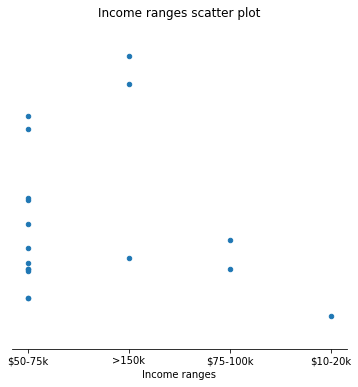
The insights can be visualized below.

fig, ax = plt.subplots(figsize=(8, 8))
output_1.plot(ax=ax, x='most common income range', y='ratio', kind='scatter', figsize=(6, 6))
ax.set_title('Income ranges scatter plot')
plt.xlabel('Income ranges')
ax.spines['right'].set_visible(False)
ax.spines['left'].set_visible(False)
ax.spines['top'].set_visible(False)
ax.get_yaxis().set_visible(False)
plt.tick_params(left=False, top=False, right=False, labelleft=False)

png

2. Visualize income distribution

fig, ax = plt.subplots(figsize=(8, 8))
pew_data.boxplot(ax=ax, rot=45)
ax.set_title('Income ranges distribution')
plt.xlabel('Income ranges')
ax.spines['right'].set_visible(False)
ax.spines['top'].set_visible(False)
ax.grid(False)
plt.tick_params(top=False, right=False)

png

pew_t = pew_data.T
pew_t

religion	Agnostic	Atheist	Buddhist	Catholic	Don’t know/refused	Evangelical Prot	Hindu	Historically Black Prot	Jehovah's Witness	Jewish	Mainline Prot	Mormon	Muslim	Orthodox	Other Christian	Other Faiths	Other World Religions	Unaffiliated
<$10k	27	12	27	418	15	575	1	228	20	19	289	29	6	13	9	20	5	217
$10-20k	34	27	21	617	14	869	9	244	27	19	495	40	7	17	7	33	2	299
$20-30k	60	37	30	732	15	1064	7	236	24	25	619	48	9	23	11	40	3	374
$30-40k	81	52	34	670	11	982	9	238	24	25	655	51	10	32	13	46	4	365
$40-50k	76	35	33	638	10	881	11	197	21	30	651	56	9	32	13	49	2	341
$50-75k	137	70	58	1116	35	1486	34	223	30	95	1107	112	23	47	14	63	7	528
$75-100k	122	73	62	949	21	949	47	131	15	69	939	85	16	38	18	46	3	407
$100-150k	109	59	39	792	17	723	48	81	11	87	753	49	8	42	14	40	4	321
>150k	84	74	53	633	18	414	54	78	6	151	634	42	6	46	12	41	4	258
Don't know/refused	96	76	54	1489	116	1529	37	339	37	162	1328	69	22	73	18	71	8	597
Total	826	515	411	8054	272	9472	257	1995	215	682	7470	581	116	363	129	449	42	3707

# drop unused columns and rows
pew_t = pew_t[1:]
pew_t = pew_t[:-2]

# make a weight table
pew_t['Total'] = pew_t.sum(axis=1)
for i in pew_t:
    pew_t[i] = pew_t[i]/pew_t['Total']*100
pew_t

religion	Agnostic	Atheist	Buddhist	Catholic	Don’t know/refused	Evangelical Prot	Hindu	Historically Black Prot	Jehovah's Witness	Jewish	Mainline Prot	Mormon	Muslim	Orthodox	Other Christian	Other Faiths	Other World Religions	Unaffiliated	Total
$10-20k	1.222582	0.970874	0.755124	22.186264	0.503416	31.247753	0.323625	8.773822	0.970874	0.683207	17.799353	1.438332	0.251708	0.611291	0.251708	1.186624	0.071917	10.751528	100.0
$20-30k	1.787310	1.102175	0.893655	21.805183	0.446828	31.694966	0.208520	7.030086	0.714924	0.744713	18.439083	1.429848	0.268097	0.685136	0.327674	1.191540	0.089366	11.140900	100.0
$30-40k	2.453059	1.574803	1.029679	20.290733	0.333131	29.739552	0.272562	7.207753	0.726832	0.757117	19.836463	1.544518	0.302847	0.969110	0.393701	1.393095	0.121139	11.053907	100.0
$40-50k	2.463533	1.134522	1.069692	20.680713	0.324149	28.557536	0.356564	6.385737	0.680713	0.972447	21.102107	1.815235	0.291734	1.037277	0.421394	1.588331	0.064830	11.053485	100.0
$50-75k	2.642237	1.350048	1.118611	21.523626	0.675024	28.659595	0.655738	4.300868	0.578592	1.832208	21.350048	2.160077	0.443587	0.906461	0.270010	1.215043	0.135005	10.183221	100.0
$75-100k	3.057644	1.829574	1.553885	23.784461	0.526316	23.784461	1.177945	3.283208	0.375940	1.729323	23.533835	2.130326	0.401003	0.952381	0.451128	1.152882	0.075188	10.200501	100.0
$100-150k	3.409446	1.845480	1.219894	24.773225	0.531749	22.614952	1.501408	2.533625	0.344073	2.721301	23.553331	1.532687	0.250235	1.313732	0.437911	1.251173	0.125117	10.040663	100.0
>150k	3.220859	2.837423	2.032209	24.271472	0.690184	15.874233	2.070552	2.990798	0.230061	5.789877	24.309816	1.610429	0.230061	1.763804	0.460123	1.572086	0.153374	9.892638	100.0

income = pew_t.index.to_list()[:-1]
pew_t_cols = pew_t.columns[:-1]
result = dict()
for i in pew_t_cols:
    result[i] = list(pew_t[i].values)

def survey(result, income):
    labels = list(result.keys())
    data = np.array(list(result.values()))
    data_cum = data.cumsum(axis=1)
    category_colors = plt.get_cmap('RdYlGn')(np.linspace(0.15, 1, data.shape[1]))

    fig, ax = plt.subplots(figsize=(10, 8))
    ax.invert_yaxis()
    ax.xaxis.set_visible(False)
    ax.set_xlim(0, np.sum(data, axis=1).max())

    for i, (colname, color) in enumerate(zip(income, category_colors)):
        widths = data[:, i]
        starts = data_cum[:, i] - widths
        ax.barh(labels, widths, left=starts, height=0.7,
                label=colname, color=color)
        # place number at center of bar
        #xcenters = starts + widths / 2

        r, g, b, _ = color
        text_color = 'white' if r * g * b < 0.5 else 'darkgrey'
        #for y, (x, c) in enumerate(zip(xcenters, widths)):
            #ax.text(x, y, str(int(c)), ha='center', va='center',
                    #color=text_color)
    ax.legend(ncol=len(income), bbox_to_anchor=(0, 1),
              loc='upper right', fontsize='large')
    ax.set_title('Income distribution per religion group')
    ax.legend()
    return fig, ax

survey(result, income)

plt.show()

png