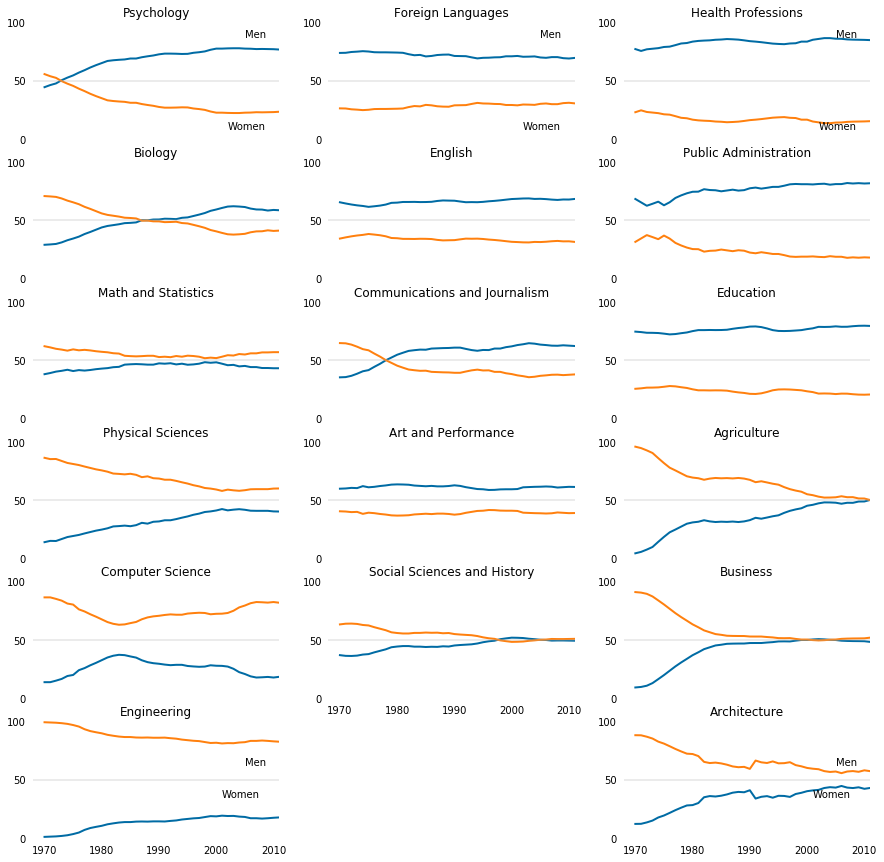
The Department of Education Statistics releases a data set annually containing the percentage of bachelor’s degrees granted to women from 1970 to 2012. The data set is broken up into 17 categories of degrees, with each column as a separate category.

Randal Olson, a data scientist at University of Pennsylvania, has cleaned the data set and made it available on his personal website.

We’ll explore how we can communicate the nuanced narrative of gender gap using effective data visualization.

import pandas as pd
import matplotlib.pyplot as plt

women_degrees = pd.read_csv('percent-bachelors-degrees-women-usa.csv')
women_degrees

	Year	Agriculture	Architecture	Art and Performance	Biology	Business	Communications and Journalism	Computer Science	Education	Engineering	English	Foreign Languages	Health Professions	Math and Statistics	Physical Sciences	Psychology	Public Administration	Social Sciences and History
0	1970	4.229798	11.921005	59.7	29.088363	9.064439	35.3	13.6	74.535328	0.8	65.570923	73.8	77.1	38.0	13.8	44.4	68.4	36.8
1	1971	5.452797	12.003106	59.9	29.394403	9.503187	35.5	13.6	74.149204	1.0	64.556485	73.9	75.5	39.0	14.9	46.2	65.5	36.2
2	1972	7.420710	13.214594	60.4	29.810221	10.558962	36.6	14.9	73.554520	1.2	63.664263	74.6	76.9	40.2	14.8	47.6	62.6	36.1
3	1973	9.653602	14.791613	60.2	31.147915	12.804602	38.4	16.4	73.501814	1.6	62.941502	74.9	77.4	40.9	16.5	50.4	64.3	36.4
4	1974	14.074623	17.444688	61.9	32.996183	16.204850	40.5	18.9	73.336811	2.2	62.413412	75.3	77.9	41.8	18.2	52.6	66.1	37.3
5	1975	18.333162	19.134048	60.9	34.449902	19.686249	41.5	19.8	72.801854	3.2	61.647206	75.0	78.9	40.7	19.1	54.5	63.0	37.7
6	1976	22.252760	21.394491	61.3	36.072871	23.430038	44.3	23.9	72.166525	4.5	62.148194	74.4	79.2	41.5	20.0	56.9	65.6	39.2
7	1977	24.640177	23.740541	62.0	38.331386	27.163427	46.9	25.7	72.456395	6.8	62.723067	74.3	80.5	41.1	21.3	59.0	69.3	40.5
8	1978	27.146192	25.849240	62.5	40.112496	30.527519	49.9	28.1	73.192821	8.4	63.619122	74.3	81.9	41.6	22.5	61.3	71.5	41.8
9	1979	29.633365	27.770477	63.2	42.065551	33.621634	52.3	30.2	73.821142	9.4	65.088390	74.2	82.3	42.3	23.7	63.3	73.3	43.6
10	1980	30.759390	28.080381	63.4	43.999257	36.765725	54.7	32.5	74.981032	10.3	65.284130	74.1	83.5	42.8	24.6	65.1	74.6	44.2
11	1981	31.318655	29.841694	63.3	45.249512	39.266230	56.4	34.8	75.845123	11.6	65.838322	73.9	84.1	43.2	25.7	66.9	74.7	44.6
12	1982	32.636664	34.816248	63.1	45.967338	41.949373	58.0	36.3	75.843649	12.4	65.847352	72.7	84.4	44.0	27.3	67.5	76.8	44.6
13	1983	31.635347	35.826257	62.4	46.713135	43.542070	58.6	37.1	75.950601	13.1	65.918380	71.8	84.6	44.3	27.6	67.9	76.1	44.1
14	1984	31.092947	35.453083	62.1	47.669083	45.124030	59.1	36.8	75.869116	13.5	65.749862	72.1	85.1	46.2	28.0	68.2	75.9	44.1
15	1985	31.379659	36.133348	61.8	47.909884	45.747782	59.0	35.7	75.923440	13.5	65.798199	70.8	85.3	46.5	27.5	69.0	75.0	43.8
16	1986	31.198719	37.240223	62.1	48.300678	46.532915	60.0	34.7	76.143015	13.9	65.982561	71.2	85.7	46.7	28.4	69.0	75.7	44.0
17	1987	31.486429	38.730675	61.7	50.209878	46.690466	60.2	32.4	76.963092	14.0	66.706031	72.0	85.5	46.5	30.4	70.1	76.4	43.9
18	1988	31.085087	39.398907	61.7	50.099811	46.764828	60.4	30.8	77.627662	13.9	67.144498	72.3	85.2	46.2	29.7	70.9	75.6	44.4
19	1989	31.612403	39.096540	62.0	50.774716	46.781565	60.5	29.9	78.111919	14.1	67.017072	72.4	84.6	46.2	31.3	71.6	76.0	44.2
20	1990	32.703444	40.824047	62.6	50.818094	47.200851	60.8	29.4	78.866859	14.1	66.921902	71.2	83.9	47.3	31.6	72.6	77.6	45.1
21	1991	34.711837	33.679881	62.1	51.468805	47.224325	60.8	28.7	78.991246	14.0	66.241475	71.1	83.5	47.0	32.6	73.2	78.2	45.5
22	1992	33.931660	35.202356	61.0	51.349742	47.219395	59.7	28.2	78.435182	14.5	65.622457	71.0	83.0	47.4	32.6	73.2	77.3	45.8
23	1993	34.946832	35.777159	60.2	51.124844	47.639332	58.7	28.5	77.267312	14.9	65.730950	70.0	82.4	46.4	33.6	73.1	78.0	46.1
24	1994	36.032674	34.433531	59.4	52.246218	47.983924	58.1	28.5	75.814933	15.7	65.641978	69.1	81.8	47.0	34.8	72.9	78.8	46.8
25	1995	36.844807	36.063218	59.2	52.599403	48.573181	58.8	27.5	75.125256	16.2	65.936949	69.6	81.5	46.1	35.9	73.0	78.8	47.9
26	1996	38.969775	35.926485	58.6	53.789880	48.647393	58.7	27.1	75.035199	16.7	66.437779	69.7	81.3	46.4	37.3	73.9	79.8	48.7
27	1997	40.685685	35.101934	58.7	54.999469	48.561050	60.0	26.8	75.163701	17.0	66.786355	70.0	81.9	47.0	38.3	74.4	81.0	49.2
28	1998	41.912403	37.598545	59.1	56.351248	49.258515	60.0	27.0	75.486160	17.8	67.255448	70.1	82.1	48.3	39.7	75.1	81.3	50.5
29	1999	42.887202	38.631529	59.2	58.228823	49.810208	61.2	28.1	75.838162	18.6	67.820221	70.9	83.5	47.8	40.2	76.5	81.1	51.2
30	2000	45.057766	40.023585	59.2	59.389857	49.803616	61.9	27.7	76.692143	18.4	68.365995	70.9	83.5	48.2	41.0	77.5	81.1	51.8
31	2001	45.866015	40.690282	59.4	60.712331	50.275145	63.0	27.6	77.375229	19.0	68.578520	71.2	85.1	47.0	42.2	77.5	80.9	51.7
32	2002	47.134658	41.132951	60.9	61.895128	50.552335	63.7	27.0	78.644244	18.7	68.829960	70.5	85.8	45.7	41.1	77.7	81.3	51.5
33	2003	47.935187	42.758543	61.1	62.169456	50.345598	64.6	25.1	78.544948	18.8	68.894487	70.6	86.5	46.0	41.7	77.8	81.5	50.9
34	2004	47.887140	43.466493	61.3	61.914587	49.950894	64.2	22.2	78.650748	18.2	68.454734	70.8	86.5	44.7	42.1	77.8	80.7	50.5
35	2005	47.672754	43.100368	61.4	61.500984	49.791851	63.4	20.6	79.067122	17.9	68.571221	69.9	86.0	45.1	41.6	77.5	81.2	50.0
36	2006	46.790300	44.499331	61.6	60.172845	49.210914	63.0	18.6	78.686306	16.8	68.297594	69.6	85.9	44.1	40.8	77.4	81.2	49.8
37	2007	47.605026	43.100459	61.4	59.411993	49.000459	62.5	17.6	78.721413	16.8	67.874923	70.2	85.4	44.1	40.7	77.1	82.1	49.3
38	2008	47.570834	42.711730	60.7	59.305765	48.888027	62.4	17.8	79.196327	16.5	67.594028	70.2	85.2	43.3	40.7	77.2	81.7	49.4
39	2009	48.667224	43.348921	61.0	58.489583	48.840474	62.8	18.1	79.532909	16.8	67.969792	69.3	85.1	43.3	40.7	77.1	82.0	49.4
40	2010	48.730042	42.066721	61.3	59.010255	48.757988	62.5	17.6	79.618625	17.2	67.928106	69.0	85.0	43.1	40.2	77.0	81.7	49.3
41	2011	50.037182	42.773438	61.2	58.742397	48.180418	62.2	18.2	79.432812	17.5	68.426730	69.5	84.8	43.1	40.1	76.7	81.9	49.2

stem_cats = ['Psychology', 'Biology', 'Math and Statistics', 'Physical Sciences', 'Computer Science', 'Engineering']
lib_arts_cats = ['Foreign Languages', 'English', 'Communications and Journalism', 'Art and Performance', 'Social Sciences and History']
other_cats = ['Health Professions', 'Public Administration', 'Education', 'Agriculture','Business', 'Architecture']

fig = plt.figure(figsize=(15, 15))

for sp in range (0, 6):
    ax = fig.add_subplot(6, 3, 3*sp+1)
    ax.plot(women_degrees['Year'], women_degrees[stem_cats[sp]], c=cb_dark_blue, label='Women', linewidth=2)
    ax.plot(women_degrees['Year'], 100-women_degrees[stem_cats[sp]], c=cb_orange, label='Men', linewidth=2)
    
    for key,spine in ax.spines.items():
        spine.set_visible(False)
    ax.set_xlim(1968, 2011)
    ax.set_ylim(0,100)
    ax.set_title(stem_cats[sp])
    ax.tick_params(bottom=False, top=False, left=False, right=False, labelbottom=False)
    ax.set_yticks([0, 50, 100])
    ax.axhline(50, c=(171/255, 171/255, 171/255), alpha=0.3)
    
    if sp == 0:
        ax.text(2005, 87, 'Men')
        ax.text(2002, 8, 'Women')
    elif sp == 5:
        ax.text(2005, 62, 'Men')
        ax.text(2001, 35, 'Women')
        ax.tick_params(labelbottom=True)
        
for sp in range (0, 5):
    ax = fig.add_subplot(6, 3, 3*sp+2)
    ax.plot(women_degrees['Year'], women_degrees[lib_arts_cats[sp]], c=cb_dark_blue, label='Women', linewidth=2)
    ax.plot(women_degrees['Year'], 100-women_degrees[lib_arts_cats[sp]], c=cb_orange, label='Men', linewidth=2)
    
    for key,spine in ax.spines.items():
        spine.set_visible(False)
    ax.set_xlim(1968, 2011)
    ax.set_ylim(0,100)
    ax.set_title(lib_arts_cats[sp])
    ax.tick_params(bottom=False, top=False, left=False, right=False, labelbottom=False)
    ax.set_yticks([0, 50, 100])
    ax.axhline(50, c=(171/255, 171/255, 171/255), alpha=0.3)
    
    if sp == 0:
        ax.text(2005, 87, 'Men')
        ax.text(2002, 8, 'Women')
    elif sp == 4:
        ax.tick_params(labelbottom=True)

for sp in range (0, 6):
    ax = fig.add_subplot(6, 3, 3*sp+3)
    ax.plot(women_degrees['Year'], women_degrees[other_cats[sp]], c=cb_dark_blue, label='Women', linewidth=2)
    ax.plot(women_degrees['Year'], 100-women_degrees[other_cats[sp]], c=cb_orange, label='Men', linewidth=2)
    
    for key,spine in ax.spines.items():
        spine.set_visible(False)
    ax.set_xlim(1968, 2011)
    ax.set_ylim(0,100)
    ax.set_title(other_cats[sp])
    ax.tick_params(bottom=False, top=False, left=False, right=False, labelbottom=False)
    ax.set_yticks([0, 50, 100])
    ax.axhline(50, c=(171/255, 171/255, 171/255), alpha=0.3)
    
    if sp == 0:
        ax.text(2005, 87, 'Men')
        ax.text(2002, 8, 'Women')
    elif sp == 5:
        ax.text(2005, 62, 'Men')
        ax.text(2001, 35, 'Women')
        ax.tick_params(labelbottom=True)
plt.savefig('gender_degrees.png')
plt.show()