Supervised learning: regression and classification of math final grades

Goals

1. Regression - final grade: MSE = 6.1558

2. Binary classification – pass if ≥ 10 else fail: 9 mis-classified points

3. 5-Level classification – based on the Erasmus grading: 7 mis-classified points

Attributes

school - student’s school (binary: ‘GP’ - Gabriel Pereira or ‘MS’ - Mousinho da Silveira)
sex - student’s sex (binary: ‘F’ - female or ‘M’ - male)
age - student’s age (numeric: from 15 to 22)
address - student’s home address type (binary: ‘U’ - urban or ‘R’ - rural)
famsize - family size (binary: ‘LE3’ - less or equal to 3 or ‘GT3’ - greater than 3)
Pstatus - parent’s cohabitation status (binary: ‘T’ - living together or ‘A’ - apart)
Medu - mother’s education (numeric: 0 - none, 1 - primary education (4th grade), 2 - 5th to 9th grade, 3 - secondary education or 4 - higher education)
Fedu - father’s education (numeric: 0 - none, 1 - primary education (4th grade), 2 - 5th to 9th grade, 3 - secondary education or 4 - higher education)
Mjob - mother’s job (nominal: ‘teacher’, ‘health’ care related, civil ‘services’ (e.g. administrative or police), ‘at_home’ or ‘other’)
Fjob - father’s job (nominal: ‘teacher’, ‘health’ care related, civil ‘services’ (e.g. administrative or police), ‘at_home’ or ‘other’)
reason - reason to choose this school (nominal: close to ‘home’, school ‘reputation’, ‘course’ preference or ‘other’)
guardian - student’s guardian (nominal: ‘mother’, ‘father’ or ‘other’)
traveltime - home to school travel time (numeric: 1 - <15 min., 2 - 15 to 30 min., 3 - 30 min. to 1 hour, or 4 - >1 hour)
studytime - weekly study time (numeric: 1 - <2 hours, 2 - 2 to 5 hours, 3 - 5 to 10 hours, or 4 - >10 hours)
failures - number of past class failures (numeric: n if 1<=n<3, else 4)
schoolsup - extra educational support (binary: yes or no)
famsup - family educational support (binary: yes or no)
paid - extra paid classes within the course subject (Math or Portuguese) (binary: yes or no)
activities - extra-curricular activities (binary: yes or no)
nursery - attended nursery school (binary: yes or no)
higher - wants to take higher education (binary: yes or no)
internet - Internet access at home (binary: yes or no)
romantic - with a romantic relationship (binary: yes or no)
famrel - quality of family relationships (numeric: from 1 - very bad to 5 - excellent)
freetime - free time after school (numeric: from 1 - very low to 5 - very high)
goout - going out with friends (numeric: from 1 - very low to 5 - very high)
Dalc - workday alcohol consumption (numeric: from 1 - very low to 5 - very high)
Walc - weekend alcohol consumption (numeric: from 1 - very low to 5 - very high)
health - current health status (numeric: from 1 - very bad to 5 - very good)
absences - number of school absences (numeric: from 0 to 93)
G1 - first period grade (numeric: from 0 to 20)
G2 - second period grade (numeric: from 0 to 20)
G3 - final grade (numeric: from 0 to 20, output target)

ML tasks

Regression - final grade G3
Binary classification – pass if G3 ≥ 10 else fail
5-Level classification – based on the Erasmus grade conversion system

import pandas as pd
import numpy as np
from sklearn.linear_model import Ridge
from sklearn.model_selection import train_test_split
from sklearn.linear_model import LinearRegression
from sklearn.linear_model import Lasso

data = pd.read_csv('student/student-mat.csv', sep=';')
data

	school	sex	age	address	famsize	Pstatus	Medu	Fedu	Mjob	Fjob	...	famrel	freetime	goout	Dalc	Walc	health	absences	G1	G2	G3
0	GP	F	18	U	GT3	A	4	4	at_home	teacher	...	4	3	4	1	1	3	6	5	6	6
1	GP	F	17	U	GT3	T	1	1	at_home	other	...	5	3	3	1	1	3	4	5	5	6
2	GP	F	15	U	LE3	T	1	1	at_home	other	...	4	3	2	2	3	3	10	7	8	10
3	GP	F	15	U	GT3	T	4	2	health	services	...	3	2	2	1	1	5	2	15	14	15
4	GP	F	16	U	GT3	T	3	3	other	other	...	4	3	2	1	2	5	4	6	10	10
...	...	...	...	...	...	...	...	...	...	...	...	...	...	...	...	...	...	...	...	...	...
390	MS	M	20	U	LE3	A	2	2	services	services	...	5	5	4	4	5	4	11	9	9	9
391	MS	M	17	U	LE3	T	3	1	services	services	...	2	4	5	3	4	2	3	14	16	16
392	MS	M	21	R	GT3	T	1	1	other	other	...	5	5	3	3	3	3	3	10	8	7
393	MS	M	18	R	LE3	T	3	2	services	other	...	4	4	1	3	4	5	0	11	12	10
394	MS	M	19	U	LE3	T	1	1	other	at_home	...	3	2	3	3	3	5	5	8	9	9

395 rows × 33 columns

Feature Engineering

o = list(data.select_dtypes(include='object').columns)
o

['school',
 'sex',
 'address',
 'famsize',
 'Pstatus',
 'Mjob',
 'Fjob',
 'reason',
 'guardian',
 'schoolsup',
 'famsup',
 'paid',
 'activities',
 'nursery',
 'higher',
 'internet',
 'romantic']

num_data = data.copy().drop(o, axis=1)

txt_data = data.loc[:, o]

# categorize these nominal features and make corresponding dummies
for i in o:
    txt_data[i] = data[i].astype('category')
    txt_data = pd.concat([txt_data, 
                        pd.get_dummies(txt_data.select_dtypes(include=['category']))], axis=1).drop(i, axis=1)

trans_data = pd.concat([txt_data, num_data], axis=1)

trans_data

	school_GP	school_MS	sex_F	sex_M	address_R	address_U	famsize_GT3	famsize_LE3	Pstatus_A	Pstatus_T	...	famrel	freetime	goout	Dalc	Walc	health	absences	G1	G2	G3
0	1	0	1	0	0	1	1	0	1	0	...	4	3	4	1	1	3	6	5	6	6
1	1	0	1	0	0	1	1	0	0	1	...	5	3	3	1	1	3	4	5	5	6
2	1	0	1	0	0	1	0	1	0	1	...	4	3	2	2	3	3	10	7	8	10
3	1	0	1	0	0	1	1	0	0	1	...	3	2	2	1	1	5	2	15	14	15
4	1	0	1	0	0	1	1	0	0	1	...	4	3	2	1	2	5	4	6	10	10
...	...	...	...	...	...	...	...	...	...	...	...	...	...	...	...	...	...	...	...	...	...
390	0	1	0	1	0	1	0	1	1	0	...	5	5	4	4	5	4	11	9	9	9
391	0	1	0	1	0	1	0	1	0	1	...	2	4	5	3	4	2	3	14	16	16
392	0	1	0	1	1	0	1	0	0	1	...	5	5	3	3	3	3	3	10	8	7
393	0	1	0	1	1	0	0	1	0	1	...	4	4	1	3	4	5	0	11	12	10
394	0	1	0	1	0	1	0	1	0	1	...	3	2	3	3	3	5	5	8	9	9

395 rows × 59 columns

1. Linear Regression (LR)

X = trans_data.iloc[:, :58].values
y = trans_data.iloc[:, 58].values

X_train, X_test, y_train, y_test = train_test_split(X, y, shuffle=True, random_state=0)

lr = LinearRegression()
lr.fit(X_train, y_train)
y_pred = lr.predict(X_test)
mse = mean_squared_error(y_test, y_pred)
mse

6.14478692382273

Regularization with Ridge Regression (RR) which sets some features to be close to zero

Try out different values of alpha for regularization

ridge_df = pd.DataFrame()
ridge_mse = []

for alpha in np.arange(1, 200, 1):
    ridge = Ridge(alpha=alpha)
    ridge.fit(X_train, y_train)
    ridge_df[alpha] = ridge.coef_
    ridge_mse.append(mean_squared_error(ridge.predict(X_test), y_test))

ridge_df = ridge_df.T
ridge_df

	0	1	2	3	4	5	6	7	8	9	...	48	49	50	51	52	53	54	55	56	57
1	-0.175165	0.175165	-0.103920	0.103920	-0.081354	0.081354	-0.056786	0.056786	0.145694	-0.145694	...	-0.157074	0.158110	0.042826	-0.061411	-0.212318	0.233830	0.094764	0.053072	0.155966	0.952054
2	-0.172091	0.172091	-0.101828	0.101828	-0.079433	0.079433	-0.056676	0.056676	0.142775	-0.142775	...	-0.157279	0.157483	0.042661	-0.061260	-0.208337	0.231553	0.094180	0.052949	0.155394	0.952180
3	-0.169075	0.169075	-0.099830	0.099830	-0.077643	0.077643	-0.056511	0.056511	0.139965	-0.139965	...	-0.157385	0.156832	0.042499	-0.061107	-0.204515	0.229363	0.093608	0.052826	0.154913	0.952247
4	-0.166125	0.166125	-0.097920	0.097920	-0.075970	0.075970	-0.056303	0.056303	0.137262	-0.137262	...	-0.157407	0.156162	0.042341	-0.060955	-0.200841	0.227253	0.093050	0.052703	0.154511	0.952261
5	-0.163244	0.163244	-0.096091	0.096091	-0.074401	0.074401	-0.056062	0.056062	0.134660	-0.134660	...	-0.157361	0.155477	0.042186	-0.060803	-0.197303	0.225217	0.092506	0.052580	0.154178	0.952231
...	...	...	...	...	...	...	...	...	...	...	...	...	...	...	...	...	...	...	...	...	...
195	-0.030416	0.030416	-0.029442	0.029442	-0.030304	0.030304	-0.023686	0.023686	0.032109	-0.032109	...	-0.098194	0.072108	0.031251	-0.043248	-0.037198	0.112158	0.055302	0.042920	0.213843	0.863639
196	-0.030254	0.030254	-0.029375	0.029375	-0.030265	0.030265	-0.023620	0.023620	0.031990	-0.031990	...	-0.098020	0.071881	0.031214	-0.043190	-0.036993	0.111923	0.055201	0.042896	0.214141	0.863209
197	-0.030093	0.030093	-0.029308	0.029308	-0.030227	0.030227	-0.023555	0.023555	0.031871	-0.031871	...	-0.097846	0.071656	0.031176	-0.043131	-0.036789	0.111688	0.055100	0.042872	0.214438	0.862781
198	-0.029933	0.029933	-0.029242	0.029242	-0.030189	0.030189	-0.023490	0.023490	0.031754	-0.031754	...	-0.097674	0.071432	0.031139	-0.043073	-0.036587	0.111456	0.055000	0.042848	0.214734	0.862353
199	-0.029774	0.029774	-0.029177	0.029177	-0.030152	0.030152	-0.023426	0.023426	0.031638	-0.031638	...	-0.097502	0.071209	0.031102	-0.043015	-0.036387	0.111224	0.054900	0.042824	0.215029	0.861926

199 rows × 58 columns

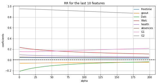
Among the last 10 features, G2 is given the highest importance, and secondly G1.

fig, ax = plt.subplots(figsize=(10, 5))
ax.plot(ridge_df.iloc[:, 50:])
ax.axhline(y=0, color='black', linestyle='--')
ax.set_xlabel("alpha")
ax.set_ylabel("coeficients")
ax.set_title("RR for the last 10 features")
ax.legend(labels=list(trans_data.iloc[:, 50:-1].columns))
ax.grid(True)

png

The plot of MSE shows the optimum alpha is in [70, 80].

fig, ax = plt.subplots(figsize=(10, 5))
plt.plot(ridge_mse)
ax.set_xlabel("alpha")
ax.set_ylabel("mse")
ax.set_title("RR MSE trace")
ax.axhline(y=mse, color='red', linestyle='--')
ax.legend(['RR', 'OLS'])
plt.show()

png

Regularization with Lasso which ignores some features completely

Try out different values of alpha for regularization. The model uses more features when alpha is smaller.

lasso_df = pd.DataFrame()
lasso_mse = []
a_range = list(reversed([1, 0.1, 0.01, 0.001, 0.0001, 0.00001, 0.000001]))
for alpha in a_range:
    lasso = Lasso(alpha=alpha, max_iter=100000)
    lasso.fit(X_train, y_train)
    print(lasso.coef_)
    lasso_df[alpha] = lasso.coef_
    lasso_mse.append(mean_squared_error(lasso.predict(X_test), y_test))

lasso_df = lasso_df.T
lasso_df

fig, ax = plt.subplots(figsize=(10, 5))
ax.plot(lasso_df.iloc[:, 50:])
ax.axhline(y=0, color='black', linestyle='--')
ax.set_xlabel("alpha")
ax.set_ylabel("coeficients")
ax.set_title("Lasso for the last 10 features")
labels = [item.get_text() for item in ax.get_xticklabels()]
for i in range(0, len(labels)-1):
    labels[i] = a_range[i] 
ax.set_xticklabels(labels, rotation=45)
ax.legend(labels=list(trans_data.iloc[:, 50:-1].columns))
ax.grid(True)

png

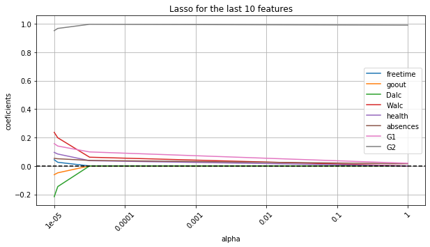
At alpha = 0.01, the model achieves the best performance which uses 42 features.

fig, ax = plt.subplots(figsize=(10, 5))
plt.plot(lasso_mse)
ax.set_xlabel("alpha")
ax.set_ylabel("mse")
ax.set_title("Lasso MSE trace")
ax.axhline(y=mse, color='red', linestyle='--')
labels = [item.get_text() for item in ax.get_xticklabels()]
for i in range(0, len(labels)-2):
    labels[i+1] = a_range[i] 
ax.set_xticklabels(labels, rotation=45)
ax.legend(['Lasso', 'OLS'])
plt.show()

png

a_001 = lasso_df.iloc[4, :]
len(a_001[a_001 != 0])

Robust Regression (RbR) for outliers

# make some strong outliers for X
X_errors = X.copy()
X_errors[::3] = 100

from sklearn.model_selection import train_test_split
X_train_error, X_test_error, y_train, y_test = train_test_split(X_errors, y, shuffle=True, random_state=0)

from sklearn.linear_model import (LinearRegression, TheilSenRegressor, RANSACRegressor, HuberRegressor)
from sklearn.metrics import mean_squared_error
estimators = [('OLS', LinearRegression()),
              ('Theil-Sen', TheilSenRegressor(random_state=42, max_iter=10000)),
              ('RANSAC', RANSACRegressor(random_state=42, max_trials=10000)),
              ('HuberRegressor', HuberRegressor(max_iter=10000))]

TheilSen is good for strong outliers, both in direction X and y.

for e in estimators:
    m = e[1].fit(X_train_error, y_train)
    print("For " + e[0] + " technique:")
    print("Training set score: {:.2f}".format(m.score(X_train_error, y_train))) 
    print("Test set score: {:.2f}".format(m.score(X_test_error, y_test))) 
    print("MSE: {:.2f} \n".format(mean_squared_error(y_test, m.predict(X_test_error))))

For OLS technique:
Training set score: 0.66
Test set score: 0.47
MSE: 15.04 

For Theil-Sen technique:
Training set score: 0.66
Test set score: 0.48
MSE: 14.73 

For RANSAC technique:
Training set score: 0.61
Test set score: 0.43
MSE: 16.09 

For HuberRegressor technique:
Training set score: 0.64
Test set score: 0.46
MSE: 15.39 

# make some strong outliers for y
y_errors = y.copy()
y_errors[::2] = 100

from sklearn.model_selection import train_test_split
X_train, X_test, y_train_error, y_test_error = train_test_split(X, y_errors, shuffle=True, random_state=0)

for e in estimators:
    m = e[1].fit(X_train, y_train_error)
    print("For " + e[0] + " technique:")
    print("Training set score: {:.2f}".format(m.score(X_train, y_train_error))) 
    print("Test set score: {:.2f}".format(m.score(X_test, y_test_error))) 
    print("MSE: {:.2f} \n".format(mean_squared_error(y_test_error, m.predict(X_test))))

For OLS technique:
Training set score: 0.10
Test set score: -0.25
MSE: 2508.31 

For Theil-Sen technique:
Training set score: 0.09
Test set score: -0.27
MSE: 2547.76 

For RANSAC technique:
Training set score: -1.51
Test set score: -2.12
MSE: 6232.98 

For HuberRegressor technique:
Training set score: 0.10
Test set score: -0.30
MSE: 2592.34 

Polynomial Regression with features G1 & G2 to predict G3

X = trans_data.iloc[:, 56:58].values
y = trans_data.iloc[:, 58].values

from sklearn.preprocessing import PolynomialFeatures
pol_mse = []
d_range = np.arange(2, 8, 1)

for d in d_range:
    pol = PolynomialFeatures(degree=d)
    pol.fit(X_train, y_train)
    X_2 = pol.fit_transform(X)
    X_train, X_test, y_train, y_test = train_test_split(X_2, y, random_state=0)
    # OLS
    lr = LinearRegression()
    lr.fit(X_train, y_train)
    y_pred = lr.predict(X_test)
    pol_mse.append(mean_squared_error(y_test, y_pred))

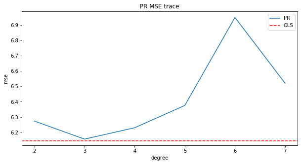
pol_mse

[6.273301123930405,
155807238512367,
229853804336613,
375376965526311,
949451552084533,
519870726895505]

Polynomial Regression with 2 features so far performs the best compared to other models

fig, ax = plt.subplots(figsize=(10, 5))
plt.plot(pol_mse)
ax.set_xlabel("degree")
ax.set_ylabel("mse")
ax.set_title("PR MSE trace")
ax.axhline(y=mse, color='red', linestyle='--')
ax.set_xticklabels(np.arange(1, 8, 1))
ax.legend(['PR', 'OLS'])
plt.show()

png

2. Binary classification for G3

Create a new column that categorizes the feature G3 as fail if < 10, and pass otherwise

def pass_grade(x):
    if x <= 10:
        return 0
    else:
        return 1
    
trans_data['pass'] = trans_data['G3'].apply(lambda x: pass_grade(x))

trans_data[['G3', 'pass']]

	G3	pass
0	6	0
1	6	0
2	10	0
3	15	1
4	10	0
...	...	...
390	9	0
391	16	1
392	7	0
393	10	0
394	9	0

395 rows × 2 columns

from sklearn.svm import LinearSVC
lsvc = LinearSVC(max_iter=100000).fit(X_train, y_train)
print("Training set score: {:.3f}".format(lsvc.score(X_train, y_train))) 
print("Test set score: {:.3f}".format(lsvc.score(X_test, y_test)))

Training set score: 0.986
Test set score: 0.899

X = trans_data.iloc[:, :58].values
y = trans_data['pass'].values

X_train, X_test, y_train, y_test = train_test_split(X, y, random_state=0) 

The model performance is best acheived when c is from 3 to 9, with 7 type-1 faults and 1 type-2 faults.

for c in list(range(1, 11)) + [100]:
    logReg = LogisticRegression(C=c, max_iter=1000000)
    logReg.fit(X_train, y_train)
    print("c is " + str(c))
    print(confusion_matrix(y_test, logReg.predict(X_test)))
    print('\n')

c is 1
[[46  5]
 [ 0 48]]


c is 2
[[46  5]
 [ 1 47]]


c is 3
[[44  7]
 [ 1 47]]


c is 4
[[44  7]
 [ 1 47]]


c is 5
[[44  7]
 [ 1 47]]


c is 6
[[44  7]
 [ 1 47]]


c is 7
[[44  7]
 [ 1 47]]


c is 8
[[44  7]
 [ 1 47]]


c is 9
[[44  7]
 [ 1 47]]


c is 10
[[43  8]
 [ 1 47]]


c is 100
[[43  8]
 [ 1 47]]

3. Multi-value classification for G3

Create a new column that categorizes the feature G3 according to ERASMUS scale

def pass_grade_5(x):
    if 0 <= x <= 9:
        return 5
    elif 10 <= x <= 11:
        return 4
    elif 12 <= x <= 13:
        return 3
    elif 14 <= x <= 15:
        return 2
    else:
        return 1
    
trans_data['pass_5'] = trans_data['G3'].apply(lambda x: pass_grade_5(x))

trans_data

	school_GP	school_MS	sex_F	sex_M	address_R	address_U	famsize_GT3	famsize_LE3	Pstatus_A	Pstatus_T	...	goout	Dalc	Walc	health	absences	G1	G2	G3	pass	pass_5
0	1	0	1	0	0	1	1	0	1	0	...	4	1	1	3	6	5	6	6	0	5
1	1	0	1	0	0	1	1	0	0	1	...	3	1	1	3	4	5	5	6	0	5
2	1	0	1	0	0	1	0	1	0	1	...	2	2	3	3	10	7	8	10	0	4
3	1	0	1	0	0	1	1	0	0	1	...	2	1	1	5	2	15	14	15	1	2
4	1	0	1	0	0	1	1	0	0	1	...	2	1	2	5	4	6	10	10	0	4
...	...	...	...	...	...	...	...	...	...	...	...	...	...	...	...	...	...	...	...	...	...
390	0	1	0	1	0	1	0	1	1	0	...	4	4	5	4	11	9	9	9	0	5
391	0	1	0	1	0	1	0	1	0	1	...	5	3	4	2	3	14	16	16	1	1
392	0	1	0	1	1	0	1	0	0	1	...	3	3	3	3	3	10	8	7	0	5
393	0	1	0	1	1	0	0	1	0	1	...	1	3	4	5	0	11	12	10	0	4
394	0	1	0	1	0	1	0	1	0	1	...	3	3	3	5	5	8	9	9	0	5

395 rows × 61 columns

X = trans_data.iloc[:, :58].values
y = trans_data['pass_5'].values

The model performance is best acheived when c is >= 8, with 6 type-1 faults and 1 type-2 faults.

for c in list(range(1, 11)) + [100]:
    lsvc = LinearSVC(C=c, max_iter=1000000)
    lsvc.fit(X_train, y_train)
    print("c is " + str(c))
    print(confusion_matrix(y_test, lsvc.predict(X_test)))
    print('\n')

c is 1
[[43  8]
 [ 2 46]]


c is 2
[[43  8]
 [ 2 46]]


c is 3
[[44  7]
 [ 2 46]]


c is 4
[[44  7]
 [ 1 47]]


c is 5
[[44  7]
 [ 1 47]]


c is 6
[[44  7]
 [ 1 47]]


c is 7
[[44  7]
 [ 1 47]]


c is 8
[[45  6]
 [ 1 47]]


c is 9
[[45  6]
 [ 1 47]]


c is 10
[[45  6]
 [ 1 47]]


c is 100
[[45  6]
 [ 1 47]]

	school_GP	school_MS	sex_F	sex_M	address_R	address_U	famsize_GT3	famsize_LE3	Pstatus_A	Pstatus_T	...	famrel	freetime	goout	Dalc	Walc	health	absences	G1	G2	G3
0	1	0	1	0	0	1	1	0	1	0	...	4	3	4	1	1	3	6	5	6	6
1	1	0	1	0	0	1	1	0	0	1	...	5	3	3	1	1	3	4	5	5	6
2	1	0	1	0	0	1	0	1	0	1	...	4	3	2	2	3	3	10	7	8	10
3	1	0	1	0	0	1	1	0	0	1	...	3	2	2	1	1	5	2	15	14	15
4	1	0	1	0	0	1	1	0	0	1	...	4	3	2	1	2	5	4	6	10	10
...	...	...	...	...	...	...	...	...	...	...	...	...	...	...	...	...	...	...	...	...	...
390	0	1	0	1	0	1	0	1	1	0	...	5	5	4	4	5	4	11	9	9	9
391	0	1	0	1	0	1	0	1	0	1	...	2	4	5	3	4	2	3	14	16	16
392	0	1	0	1	1	0	1	0	0	1	...	5	5	3	3	3	3	3	10	8	7
393	0	1	0	1	1	0	0	1	0	1	...	4	4	1	3	4	5	0	11	12	10
394	0	1	0	1	0	1	0	1	0	1	...	3	2	3	3	3	5	5	8	9	9

	school_GP	school_MS	sex_F	sex_M	address_R	address_U	famsize_GT3	famsize_LE3	Pstatus_A	Pstatus_T	...	goout	Dalc	Walc	health	absences	G1	G2	G3	pass	pass_5
0	1	0	1	0	0	1	1	0	1	0	...	4	1	1	3	6	5	6	6	0	5
1	1	0	1	0	0	1	1	0	0	1	...	3	1	1	3	4	5	5	6	0	5
2	1	0	1	0	0	1	0	1	0	1	...	2	2	3	3	10	7	8	10	0	4
3	1	0	1	0	0	1	1	0	0	1	...	2	1	1	5	2	15	14	15	1	2
4	1	0	1	0	0	1	1	0	0	1	...	2	1	2	5	4	6	10	10	0	4
...	...	...	...	...	...	...	...	...	...	...	...	...	...	...	...	...	...	...	...	...	...
390	0	1	0	1	0	1	0	1	1	0	...	4	4	5	4	11	9	9	9	0	5
391	0	1	0	1	0	1	0	1	0	1	...	5	3	4	2	3	14	16	16	1	1
392	0	1	0	1	1	0	1	0	0	1	...	3	3	3	3	3	10	8	7	0	5
393	0	1	0	1	1	0	0	1	0	1	...	1	3	4	5	0	11	12	10	0	4
394	0	1	0	1	0	1	0	1	0	1	...	3	3	3	5	5	8	9	9	0	5

	school_GP	school_MS	sex_F	sex_M	address_R	address_U	famsize_GT3	famsize_LE3	Pstatus_A	Pstatus_T	...	famrel	freetime	goout	Dalc	Walc	health	absences	G1	G2	G3
0	1	0	1	0	0	1	1	0	1	0	...	4	3	4	1	1	3	6	5	6	6
1	1	0	1	0	0	1	1	0	0	1	...	5	3	3	1	1	3	4	5	5	6
2	1	0	1	0	0	1	0	1	0	1	...	4	3	2	2	3	3	10	7	8	10
3	1	0	1	0	0	1	1	0	0	1	...	3	2	2	1	1	5	2	15	14	15
4	1	0	1	0	0	1	1	0	0	1	...	4	3	2	1	2	5	4	6	10	10
...	...	...	...	...	...	...	...	...	...	...	...	...	...	...	...	...	...	...	...	...	...
390	0	1	0	1	0	1	0	1	1	0	...	5	5	4	4	5	4	11	9	9	9
391	0	1	0	1	0	1	0	1	0	1	...	2	4	5	3	4	2	3	14	16	16
392	0	1	0	1	1	0	1	0	0	1	...	5	5	3	3	3	3	3	10	8	7
393	0	1	0	1	1	0	0	1	0	1	...	4	4	1	3	4	5	0	11	12	10
394	0	1	0	1	0	1	0	1	0	1	...	3	2	3	3	3	5	5	8	9	9

	school_GP	school_MS	sex_F	sex_M	address_R	address_U	famsize_GT3	famsize_LE3	Pstatus_A	Pstatus_T	...	goout	Dalc	Walc	health	absences	G1	G2	G3	pass	pass_5
0	1	0	1	0	0	1	1	0	1	0	...	4	1	1	3	6	5	6	6	0	5
1	1	0	1	0	0	1	1	0	0	1	...	3	1	1	3	4	5	5	6	0	5
2	1	0	1	0	0	1	0	1	0	1	...	2	2	3	3	10	7	8	10	0	4
3	1	0	1	0	0	1	1	0	0	1	...	2	1	1	5	2	15	14	15	1	2
4	1	0	1	0	0	1	1	0	0	1	...	2	1	2	5	4	6	10	10	0	4
...	...	...	...	...	...	...	...	...	...	...	...	...	...	...	...	...	...	...	...	...	...
390	0	1	0	1	0	1	0	1	1	0	...	4	4	5	4	11	9	9	9	0	5
391	0	1	0	1	0	1	0	1	0	1	...	5	3	4	2	3	14	16	16	1	1
392	0	1	0	1	1	0	1	0	0	1	...	3	3	3	3	3	10	8	7	0	5
393	0	1	0	1	1	0	0	1	0	1	...	1	3	4	5	0	11	12	10	0	4
394	0	1	0	1	0	1	0	1	0	1	...	3	3	3	5	5	8	9	9	0	5

	school_GP	school_MS	sex_F	sex_M	address_R	address_U	famsize_GT3	famsize_LE3	Pstatus_A	Pstatus_T	...	famrel	freetime	goout	Dalc	Walc	health	absences	G1	G2	G3
0	1	0	1	0	0	1	1	0	1	0	...	4	3	4	1	1	3	6	5	6	6
1	1	0	1	0	0	1	1	0	0	1	...	5	3	3	1	1	3	4	5	5	6
2	1	0	1	0	0	1	0	1	0	1	...	4	3	2	2	3	3	10	7	8	10
3	1	0	1	0	0	1	1	0	0	1	...	3	2	2	1	1	5	2	15	14	15
4	1	0	1	0	0	1	1	0	0	1	...	4	3	2	1	2	5	4	6	10	10
...	...	...	...	...	...	...	...	...	...	...	...	...	...	...	...	...	...	...	...	...	...
390	0	1	0	1	0	1	0	1	1	0	...	5	5	4	4	5	4	11	9	9	9
391	0	1	0	1	0	1	0	1	0	1	...	2	4	5	3	4	2	3	14	16	16
392	0	1	0	1	1	0	1	0	0	1	...	5	5	3	3	3	3	3	10	8	7
393	0	1	0	1	1	0	0	1	0	1	...	4	4	1	3	4	5	0	11	12	10
394	0	1	0	1	0	1	0	1	0	1	...	3	2	3	3	3	5	5	8	9	9

	school_GP	school_MS	sex_F	sex_M	address_R	address_U	famsize_GT3	famsize_LE3	Pstatus_A	Pstatus_T	...	goout	Dalc	Walc	health	absences	G1	G2	G3	pass	pass_5
0	1	0	1	0	0	1	1	0	1	0	...	4	1	1	3	6	5	6	6	0	5
1	1	0	1	0	0	1	1	0	0	1	...	3	1	1	3	4	5	5	6	0	5
2	1	0	1	0	0	1	0	1	0	1	...	2	2	3	3	10	7	8	10	0	4
3	1	0	1	0	0	1	1	0	0	1	...	2	1	1	5	2	15	14	15	1	2
4	1	0	1	0	0	1	1	0	0	1	...	2	1	2	5	4	6	10	10	0	4
...	...	...	...	...	...	...	...	...	...	...	...	...	...	...	...	...	...	...	...	...	...
390	0	1	0	1	0	1	0	1	1	0	...	4	4	5	4	11	9	9	9	0	5
391	0	1	0	1	0	1	0	1	0	1	...	5	3	4	2	3	14	16	16	1	1
392	0	1	0	1	1	0	1	0	0	1	...	3	3	3	3	3	10	8	7	0	5
393	0	1	0	1	1	0	0	1	0	1	...	1	3	4	5	0	11	12	10	0	4
394	0	1	0	1	0	1	0	1	0	1	...	3	3	3	5	5	8	9	9	0	5